使用python的plot绘制loss、acc曲线,并存储成图片 |
您所在的位置:网站首页 › 如何画二次函数图像的过程图 › 使用python的plot绘制loss、acc曲线,并存储成图片 |
使用python的plot绘制loss、acc曲线,并存储成图片
|
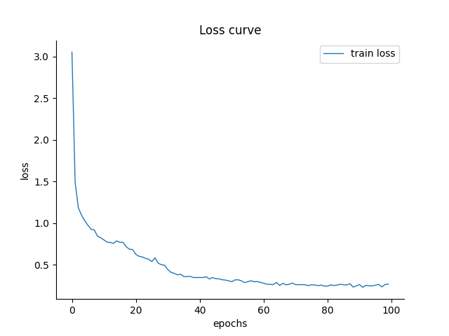
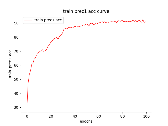
使用 python的plot 绘制网络训练过程中的的 loss 曲线以及准确率变化曲线,这里的主要思想就时先把想要的损失值以及准确率值保存下来,保存到 .txt 文件中,待网络训练结束,我们再拿这存储的数据绘制各种曲线。 其大致步骤为:数据读取与存储 - > loss曲线绘制 - > 准确率曲线绘制 一、数据读取与存储部分我们首先要得到训练时的数据,以损失值为例,网络每迭代一次都会产生相应的 loss,那么我们就把每一次的损失值都存储下来,存储到列表,保存到 .txt 文件中。 1.3817585706710815, 1.8422836065292358, 1.1619832515716553, 0.5217241644859314, 0.5221078991889954, 1.3544578552246094, 1.3334463834762573, 1.3866571187973022, 0.7603049278259277上图为部分损失值,根据迭代次数而异,要是迭代了1万次,这里就会有1万个损失值。 而准确率值是每一个 epoch 产生一个值,要是训练100个epoch,就有100个准确率值。 这里的损失值是怎么保存到文件中的呢?首先,找到网络训练代码,就是项目中的 main.py,或者 train.py ,在文件里先找到训练部分,里面经常会有这样一行代码: for epoch in range(resume_epoch, num_epochs): # 就是这一行 #### ... loss = criterion(outputs, labels.long()) # 损失样例 ... epoch_acc = running_corrects.double() / trainval_sizes[phase] # 准确率样例 ... ###从这一行开始就是训练部分了,往下会找到类似的这两句代码,就是损失值和准确率值了。 这时候将以下代码加入源代码就可以了: train_loss = [] train_acc = [] for epoch in range(resume_epoch, num_epochs): # 就是这一行 ### ... loss = criterion(outputs, labels.long()) # 损失样例 train_loss.append(loss.item()) # 损失加入到列表中 ... epoch_acc = running_corrects.double() / trainval_sizes[phase] # 准确率样例 train_acc.append(epoch_acc.item()) # 准确率加入到列表中 ... with open("./train_loss.txt", 'w') as train_los: train_los.write(str(train_loss)) with open("./train_acc.txt", 'w') as train_ac: train_ac.write(str(train_acc))这样就算完成了损失值和准确率值的数据存储了! 二、绘制 loss 曲线主要需要 numpy 库和 matplotlib 库。 pip install numpy malplotlib首先,将 .txt 文件中的存储的数据读取进来,以下是读取函数: import numpy as np # 读取存储为txt文件的数据 def data_read(dir_path): with open(dir_path, "r") as f: raw_data = f.read() data = raw_data[1:-1].split(", ") # [-1:1]是为了去除文件中的前后中括号"[]" return np.asfarray(data, float)然后,就是绘制 loss 曲线部分: if __name__ == "__main__": train_loss_path = r"/train_loss.txt" # 存储文件路径 y_train_loss = data_read(train_loss_path) # loss值,即y轴 x_train_loss = range(len(y_train_loss)) # loss的数量,即x轴 plt.figure() # 去除顶部和右边框框 ax = plt.axes() ax.spines['top'].set_visible(False) ax.spines['right'].set_visible(False) plt.xlabel('iters') # x轴标签 plt.ylabel('loss') # y轴标签 # 以x_train_loss为横坐标,y_train_loss为纵坐标,曲线宽度为1,实线,增加标签,训练损失, # 默认颜色,如果想更改颜色,可以增加参数color='red',这是红色。 plt.plot(x_train_loss, y_train_loss, linewidth=1, linestyle="solid", label="train loss") plt.legend() plt.title('Loss curve') plt.show() pit.savefig("loss.png")这样就算把损失图像画出来了!如下: 三、绘制准确率曲线 有了上面的基础,这就简单很多了。 只是有一点要记住,上面的x轴是迭代次数,这里的是训练轮次 epoch。 if __name__ == "__main__": train_acc_path = r"/train_acc.txt" # 存储文件路径 y_train_acc = data_read(train_acc_path) # 训练准确率值,即y轴 x_train_acc = range(len(y_train_acc)) # 训练阶段准确率的数量,即x轴 plt.figure() # 去除顶部和右边框框 ax = plt.axes() ax.spines['top'].set_visible(False) ax.spines['right'].set_visible(False) plt.xlabel('epochs') # x轴标签 plt.ylabel('accuracy') # y轴标签 # 以x_train_acc为横坐标,y_train_acc为纵坐标,曲线宽度为1,实线,增加标签,训练损失, # 增加参数color='red',这是红色。 plt.plot(x_train_acc, y_train_acc, color='red',linewidth=1, linestyle="solid", label="train acc") plt.legend() plt.title('Accuracy curve') plt.show() pit.savefig("acc.png")这样就把准确率变化曲线画出来了!如下: 以下是完整代码,以绘制准确率曲线为例,并且将x轴换成了iters,和损失曲线保持一致,供参考: import numpy as np import matplotlib.pyplot as plt # 读取存储为txt文件的数据 def data_read(dir_path): with open(dir_path, "r") as f: raw_data = f.read() data = raw_data[1:-1].split(", ") return np.asfarray(data, float) # 不同长度数据,统一为一个标准,倍乘x轴 def multiple_equal(x, y): x_len = len(x) y_len = len(y) times = x_len/y_len y_times = [i * times for i in y] return y_times if __name__ == "__main__": train_loss_path = r"/train_loss.txt" train_acc_path = r"/train_acc.txt" y_train_loss = data_read(train_loss_path) y_train_acc = data_read(train_acc_path) x_train_loss = range(len(y_train_loss)) x_train_acc = multiple_equal(x_train_loss, range(len(y_train_acc))) plt.figure() # 去除顶部和右边框框 ax = plt.axes() ax.spines['top'].set_visible(False) ax.spines['right'].set_visible(False) plt.xlabel('iters') plt.ylabel('accuracy') # plt.plot(x_train_loss, y_train_loss, linewidth=1, linestyle="solid", label="train loss") plt.plot(x_train_acc, y_train_acc, color='red', linestyle="solid", label="train accuracy") plt.legend() plt.title('Accuracy curve') plt.show() pit.savefig("acc.png") |
【本文地址】
今日新闻 |
推荐新闻 |