使用 gnuplot 进行数据拟合(输出的含义是什么?) |
您所在的位置:网站首页 › 多自变量拟合什么意思啊 › 使用 gnuplot 进行数据拟合(输出的含义是什么?) |
使用 gnuplot 进行数据拟合(输出的含义是什么?)
|
这里给出使用 gnuplot 进行数据拟合的一个实例。 待拟合的数据如下。文件名:data.dat。 0.000000 -2618.996712 0.010000 -2618.996666 0.020000 -2618.996516 0.030000 -2618.996266 0.040000 -2618.995922 0.050000 -2618.995509我已经知道这一组数据是一条抛物线(y=ax^2+bx+c),并且系数 b 是 0,因此此处我可以作线性拟合,即以 x^2 为自变量,y 为因变量。 TODO: 考虑到 x^2 和 y 的数量级相差很大,为了拟合过程比较稳定,我应该对 y 进行平移,即将 y 减去 y_min,其中 y_min 是 y 的最小值。但是不知道怎么在 gnuplot 里面实现(这在 Python 里面很容易)。 gnuplot 脚本如下。文件名:linear_fit.gpi。注意, 采用 gpi 作为gnuplot 脚本的后缀的好处在于 vim 可以对其进行语法高亮。 # 设置输出文件名和格式 # set terminal png size 600, 400 font "Arial, 12" # set output 'linear_fit.png' set terminal postscript set output 'linear_fit.ps' set border linewidth 0.5 set format "%0.2e" set tics out # 设置坐标轴标签 set xlabel 'X**2' set ylabel 'Y' set title 'Data and Linear Fit' set grid filename = 'data.dat' # Linear fit f(x) = a*x + b fit f(x) filename using ($1**2):2 via a, b # 绘制数据散点图 plot filename using ($1**2):2 title 'Data' with points, \ f(x) title 'Linear Fit' with lines # 显示图例 set key outside # 刷新绘图 replot # 保存绘图 set output在终端中执行上述脚本,得到的结果如下。 $ gnuplot linear_fit.gpi iter chisq delta/lim lambda a b 0 4.1186311397e+07 0.00e+00 7.07e-01 1.000000e+00 1.000000e+00 1 2.4370634067e+05 -1.68e+07 7.07e-02 -1.216903e+00 -2.417457e+03 2 1.6897591839e-01 -1.44e+11 7.07e-03 -1.399703e+00 -2.618827e+03 3 1.4055900272e-05 -1.20e+09 7.07e-04 -1.236468e+00 -2.618995e+03 4 1.2792113431e-07 -1.09e+07 7.07e-05 3.201171e-01 -2.618997e+03 5 3.5201131736e-10 -3.62e+07 7.07e-06 4.838535e-01 -2.618997e+03 6 3.5187012685e-10 -4.01e+01 7.07e-07 4.840260e-01 -2.618997e+03 7 3.5187012297e-10 -1.10e-03 7.07e-08 4.840260e-01 -2.618997e+03 iter chisq delta/lim lambda a b After 7 iterations the fit converged. final sum of squares of residuals : 3.5187e-10 rel. change during last iteration : -1.10104e-08 degrees of freedom (FIT_NDF) : 4 rms of residuals (FIT_STDFIT) = sqrt(WSSR/ndf) : 9.3791e-06 variance of residuals (reduced chisquare) = WSSR/ndf : 8.79675e-11 Final set of parameters Asymptotic Standard Error ======================= ========================== a = 0.484026 +/- 0.004304 (0.8892%) b = -2619 +/- 5.498e-06 (2.099e-07%) correlation matrix of the fit parameters: a b a 1.000 b -0.718 1.000上述输出还会缀加写入当前目录下面的 fit.log 文件,以备查。 同时,生成的 linear_fit.ps 文件是绘制的图形。如果不能直接查看的话,可以使用下面的命令将其转换为 pdf 文件。 $ ps2pdf linear_fit.ps绘制的图像如下。 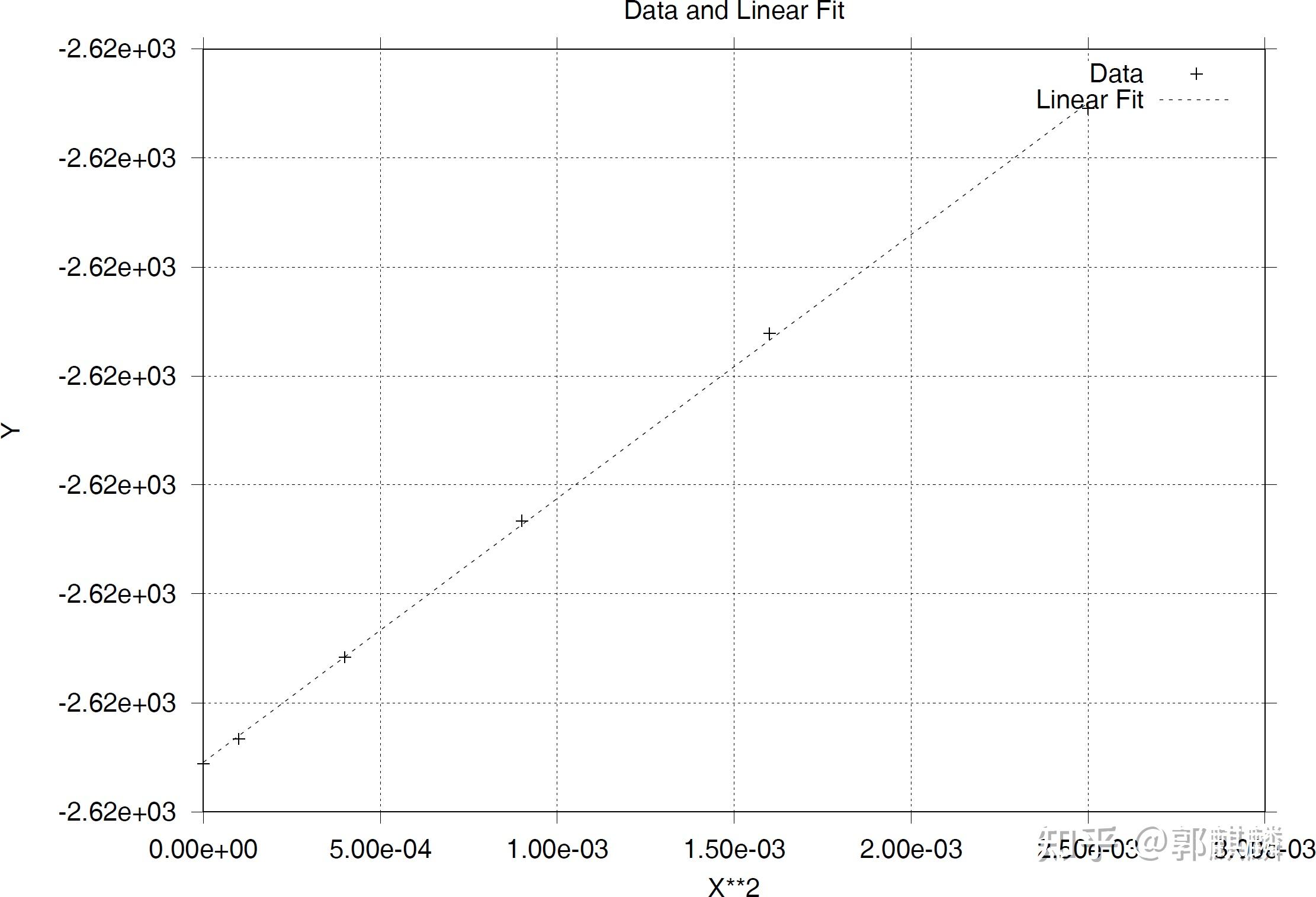 原始数据和拟合以后的数据的图像 原始数据和拟合以后的数据的图像问题: degrees of freedom (FIT_NDF) 是什么意思? 有什么意义? rms of residuals (FIT_STDFIT) = sqrt(WSSR/ndf) 是什么意思?有什么意义? variance of residuals (reduced chisquare) = WSSR/ndf 是什么意思? 有什么意义? 拟合结果中的 correlation matrix of the fit parameters 是怎么得到的?算法是什么?有什么意义? 使用 scipy.optimize 提供的 leastsq(最小二乘法)拟合的 Python 代码如下。文件名:linear_fit_v1.py。 import numpy as np from scipy.optimize import leastsq from matplotlib import pyplot as plt # 定义线性模型函数 def linear_func(params, x): a, b = params return a * x + b # 定义误差函数 def residuals(params, y, x): return y - linear_func(params, x) # 读取数据文件 data_file = 'data.dat' data = np.loadtxt(data_file) x0 = data[0:, 0] y0 = data[0:, 1] y_min = np.min(y0) x = x0 ** 2 y = y0 - y_min # 初始拟合参数估计 initial_params = [1.0, 1.0] # 使用 leastsq 进行线性拟合 params, _ = leastsq(func=residuals, x0=initial_params, args=(y, x)) # 提取拟合参数 a, b = params # 预测值 y_pred = linear_func(params, x) res= y - y_pred # 残差 rms = np.sqrt(np.mean(res ** 2)) print('RMS of residuals:', rms) # 计算拟合优度信息 SSR = np.sum(res ** 2) # 残差的平方和 SST = np.sum((y - np.mean(y)) ** 2) # 总平方和 r_squared = 1 - SSR/SST # 拟合优度 print("a =", a) print("b =", b + y_min) print("SSR = %0.4e" % SSR) print("SST = %0.4e" % SST) print("拟合优度 (R-squared):", r_squared) # 绘图 fig = plt.figure(figsize=(6, 4), dpi=100) p1 = plt.scatter(x=x, y=y, label='Data') p2 = plt.plot(x, y_pred, color='r', label='Linear fit') plt.gca().xaxis.set_major_formatter(plt.FormatStrFormatter('%0.2e')) plt.xlabel('x ** 2') plt.ylabel('y') plt.legend() plt.grid(True) plt.show()上述脚本的执行结果如下。 RMS of residuals: 6.604392147478035e-06 a = 1.915008774843253 b = -2618.99671942471 SSR = 2.6171e-10 SST = 1.7414e-05 拟合优度 (R-squared): 0.9999849710827738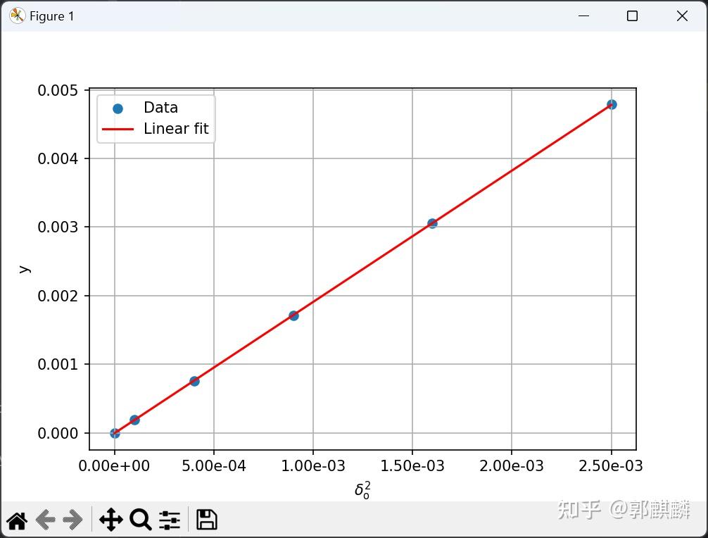 写于 2023/06/16 经查阅 gnuplot 手册,现在知道了相关参数是怎么得到的了。Python 代码如下。文件名:linear_fit_v2.py。 import numpy as np from scipy.optimize import leastsq from matplotlib import pyplot as plt # 定义线性模型函数 def linear_func(fit_params, x_data): param_a, param_b = fit_params return param_a * x_data + param_b # 定义误差函数 def residuals(fit_params, y_data, x_data): return y_data - linear_func(fit_params, x_data) # 读取数据文件 data_file = 'data.dat' data = np.loadtxt(data_file) x0 = data[0:, 0] y0 = data[0:, 1] y_min = np.min(y0) x = x0 ** 2 y = y0 - y_min # 初始拟合参数估计 initial_params = [1.0, 1.0] # 使用 leastsq 进行线性拟合 # params, _ = leastsq(func=residuals, x0=initial_params, args=(y, x), full_output=False) [p_opt, cov_x, info_dict, msg, ier] = leastsq(func=residuals, x0=initial_params, args=(y, x), full_output=True) # 提取拟合参数 a, b = p_opt # 注意!前面平移了,拟合以后要加回来。仅限于线性拟合。 b += y_min # 预测值 y_pred = linear_func(p_opt, x) res = y - y_pred # 残差 # 计算拟合优度信息 ssr = np.sum(res ** 2) # 残差的平方和 sst = np.sum((y - np.mean(y)) ** 2) # 总平方和 r_squared = 1 - ssr / sst # 拟合优度 print("a:".rjust(30), a) print("b:".rjust(30), b) print("SSR:".rjust(30), ssr) print("SST:".rjust(30), sst) print("R-squared:".rjust(30), r_squared) num_data = len(x0) # 数据点的个数 num_params = 2 # 拟合参数的个数 (a, b) ndf = num_data - num_params # Number of degrees of freedom # See gnuplot 5.4 manual, page 94 wssr = np.sum(res ** 2) # Weighted sum-of-squares residual reduced_chi_squared = wssr / ndf stdfit = np.sqrt(reduced_chi_squared) print("degrees of freedom:".rjust(30), ndf) print('rms of residuals:'.rjust(30), stdfit) print("variance of residuals:".rjust(30), reduced_chi_squared) # 计算协方差矩阵 (): cov_x --> p_cov n = len(p_opt) m = len(x) J = np.zeros((m, n)) for i in range(n): params_perturbed = p_opt.copy() params_perturbed[i] += np.sqrt(np.finfo(float).eps) * p_opt[i] J[:, i] = (residuals(params_perturbed, y, x) - residuals(p_opt, y, x)) / np.sqrt(np.finfo(float).eps) / p_opt[i] residual_variance = np.sum(residuals(p_opt, y, x) ** 2) / (m - n) p_cov = residual_variance * np.linalg.inv(J.T @ J) # 获取参数估计值的渐近标准误差 (Asymptotic Standard Error) p_err = np.sqrt(np.diag(p_cov)) print("a:".rjust(30) + "%25.15f +/- %0.15e" % (a, p_err[0])) print("b:".rjust(30) + "%25.15f +/- %0.15e" % (b, p_err[1])) correlation_matrix = p_cov / np.outer(p_err, p_err) # np.outer(a, b): direct product of a and b print("拟合参数的协方差矩阵:") print(p_cov) print("correlation matrix of the fit parameters:") print(correlation_matrix) # 绘图 fig = plt.figure(figsize=(6, 4), dpi=100) p1 = plt.scatter(x=x, y=y, label='Data') p2 = plt.plot(x, y_pred, color='r', label='Linear fit') plt.gca().xaxis.set_major_formatter(plt.FormatStrFormatter('%0.2e')) plt.xlabel('$x^{2}$') plt.ylabel('y') plt.legend() plt.grid(True) plt.savefig(fname='linear_fit.pdf', format='pdf') plt.show()上述代码的执行结果与 gnuplot 的执行结果比较如下。 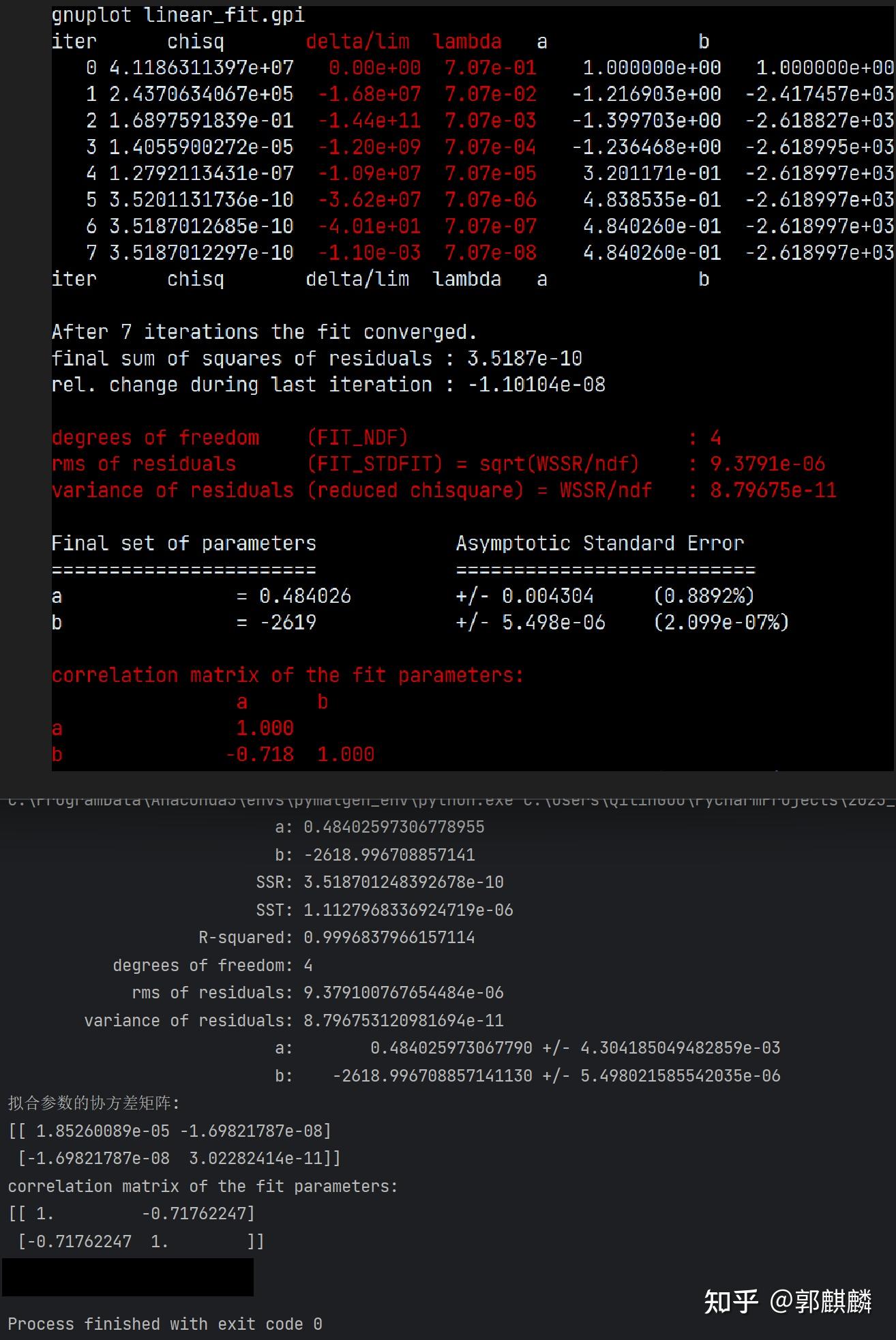 2023/06/20 星期二 |
【本文地址】
今日新闻 |
推荐新闻 |