基于机器学习进行降雨预测 |
您所在的位置:网站首页 › 论述空间分析方法如何解决预测和预报的问题 › 基于机器学习进行降雨预测 |
基于机器学习进行降雨预测
|
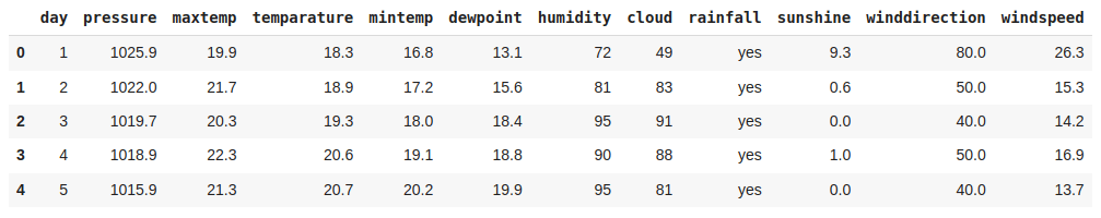
在本文中,我们将学习如何构建一个机器学习模型,该模型可以根据一些大气因素预测今天是否会有降雨。这个问题与使用机器学习的降雨预测有关,因为机器学习模型往往在以前已知的任务上表现得更好,而这些任务需要高技能的个人来完成。 导入库和数据集Python库使我们可以轻松地处理数据,并通过一行代码执行典型和复杂的任务。 Pandas -此库有助于以2D阵列格式加载数据帧,并具有多种功能,可一次性执行分析任务。Numpy - Numpy数组非常快,可以在很短的时间内执行大型计算。Matplotlib/Seaborn -这个库用于绘制可视化。Sklearn -此模块包含多个库,这些库具有预实现的功能,以执行从数据预处理到模型开发和评估的任务。XGBoost -这包含eXtreme Gradient Boosting机器学习算法,这是帮助我们实现高精度预测的算法之一。Imblearn -此模块包含一个函数,可用于处理与数据不平衡相关的问题。 import numpy as np import pandas as pd import matplotlib.pyplot as plt import seaborn as sb from sklearn.model_selection import train_test_split from sklearn.preprocessing import StandardScaler from sklearn import metrics from sklearn.svm import SVC from xgboost import XGBClassifier from sklearn.linear_model import LogisticRegression from imblearn.over_sampling import RandomOverSampler import warnings warnings.filterwarnings('ignore')现在,让我们将数据集加载到panda的数据框中,并打印它的前五行。 df = pd.read_csv('Rainfall.csv') df.head()
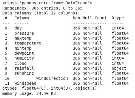
输出: (366, 12) df.info()
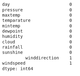
从原始数据源获得的数据被称为原始数据,在我们可以从中得出任何结论或对其进行建模之前需要大量的预处理。这些预处理步骤被称为数据清理,它包括离群值删除,空值插补,以及删除数据输入中的任何类型的差异。 df.isnull().sum()
输出: Index(['day', 'pressure ', 'maxtemp', 'temperature', 'mintemp', 'dewpoint', 'humidity ', 'cloud ', 'rainfall', 'sunshine', ' winddirection', 'windspeed'], dtype='object')在这里我们可以观察到在列名中有不必要的空格,让我们删除它。 df.rename(str.strip, axis='columns', inplace=True) df.columns输出: Index(['day', 'pressure', 'maxtemp', 'temperature', 'mintemp', 'dewpoint', 'humidity', 'cloud', 'rainfall', 'sunshine', 'winddirection', 'windspeed'], dtype='object')现在是时候进行空值填充了。 for col in df.columns: # Checking if the column contains # any null values if df[col].isnull().sum() > 0: val = df[col].mean() df[col] = df[col].fillna(val) df.isnull().sum().sum()输出: 0 探索性数据分析EDA是一种使用可视化技术分析数据的方法。它用于发现趋势和模式,或在统计摘要和图形表示的帮助下检查假设。在这里,我们将看到如何检查数据的不平衡和偏斜。 plt.pie(df['rainfall'].value_counts().values, labels = df['rainfall'].value_counts().index, autopct='%1.1f%%') plt.show()
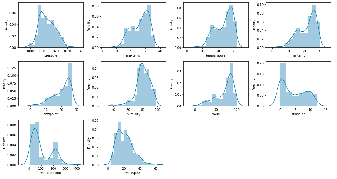
在这里我们可以清楚地得出一些观察结果: 在降雨的日子,maxtemp相对较低。降水日dewpoint 值较高。在预计会下雨的日子里humidity 很高。显然,cloud 与降雨相关性大。降雨日的sunshine亦较少。降雨日windspeed 较高。我们从上述数据集中得出的观察结果与真实的生活中观察到的非常相似。 features = list(df.select_dtypes(include = np.number).columns) features.remove('day') print(features)输出: ['pressure', 'maxtemp', 'temperature', 'mintemp', 'dewpoint', 'humidity', 'cloud', 'sunshine', 'winddirection', 'windspeed']让我们检查数据集中给定的连续特征的分布。 plt.subplots(figsize=(15,8)) for i, col in enumerate(features): plt.subplot(3,4, i + 1) sb.distplot(df[col]) plt.tight_layout() plt.show()
有时,存在高度相关的特征,这些特征只是增加了特征空间的维度,对模型的性能没有好处。因此,我们必须检查该数据集中是否存在高度相关的特征。 plt.figure(figsize=(10,10)) sb.heatmap(df.corr() > 0.8, annot=True, cbar=False) plt.show()
现在,我们将分离特征和目标变量,并将它们分成训练和测试数据,我们将使用这些数据来选择在验证数据上表现最好的模型。 features = df.drop(['day', 'rainfall'], axis=1) target = df.rainfall正如我们之前发现的那样,我们使用的数据集是不平衡的,因此,我们必须在将其输入模型之前平衡训练数据。 X_train, X_val, \ Y_train, Y_val = train_test_split(features, target, test_size=0.2, stratify=target, random_state=2) # As the data was highly imbalanced we will # balance it by adding repetitive rows of minority class. ros = RandomOverSampler(sampling_strategy='minority', random_state=22) X, Y = ros.fit_resample(X_train, Y_train)数据集的特征在不同的尺度上,因此在训练之前对其进行归一化将有助于我们更快地获得最佳结果。 # Normalizing the features for stable and fast training. scaler = StandardScaler() X = scaler.fit_transform(X) X_val = scaler.transform(X_val)现在,让我们训练一些最先进的分类模型,并在我们的训练数据上训练它们。 models = [LogisticRegression(), XGBClassifier(), SVC(kernel='rbf', probability=True)] for i in range(3): models[i].fit(X, Y) print(f'{models[i]} : ') train_preds = models[i].predict_proba(X) print('Training Accuracy : ', metrics.roc_auc_score(Y, train_preds[:,1])) val_preds = models[i].predict_proba(X_val) print('Validation Accuracy : ', metrics.roc_auc_score(Y_val, val_preds[:,1]))输出: LogisticRegression() : Training Accuracy : 0.8893967324057472 Validation Accuracy : 0.8966666666666667 XGBClassifier() : Training Accuracy : 0.9903285270573975 Validation Accuracy : 0.8408333333333333 SVC(probability=True) : Training Accuracy : 0.9026413474407211 Validation Accuracy : 0.8858333333333333 模型评估从以上准确度来看,我们可以说逻辑回归和支持向量分类器是令人满意的,因为训练和验证准确度之间的差距很低。让我们使用SVC模型绘制验证数据的混淆矩阵。 metrics.plot_confusion_matrix(models[2], X_val, Y_val) plt.show()
输出: precision recall f1-score support 0 0.84 0.67 0.74 24 1 0.85 0.94 0.90 50 accuracy 0.85 74 macro avg 0.85 0.80 0.82 74 weighted avg 0.85 0.85 0.85 74 |
 根据上述关于每列中数据的信息,我们可以观察到没有空值。
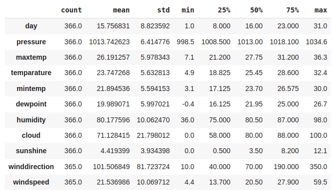
 因此,在“winddirection”和“windspeed”列中存在一个空值。但"风向“这一栏是怎么回事?
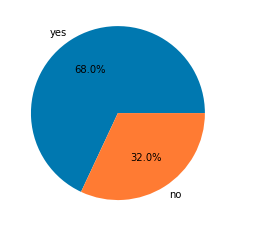
 让我们为连续变量绘制箱形图,以检测数据中存在的异常值。
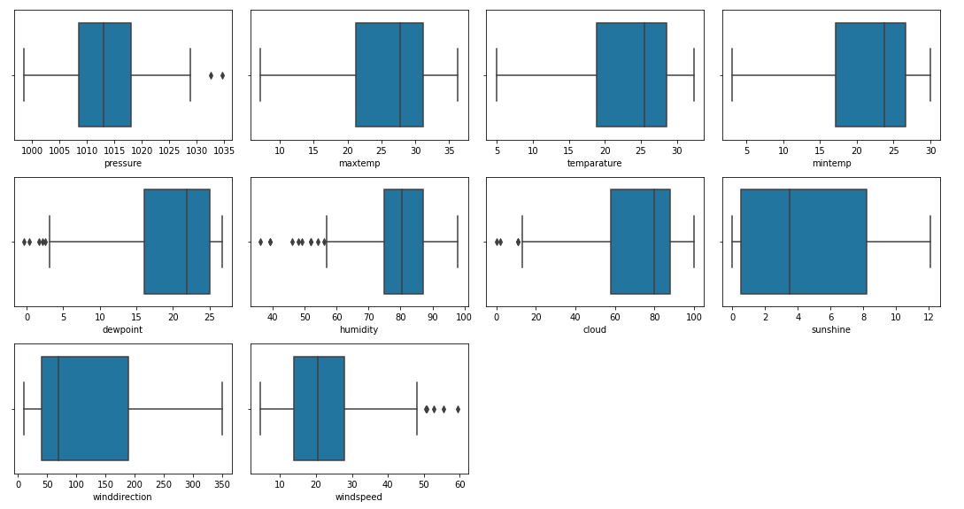 数据中有异常值,但遗憾的是我们没有太多数据,因此我们无法删除此数据。
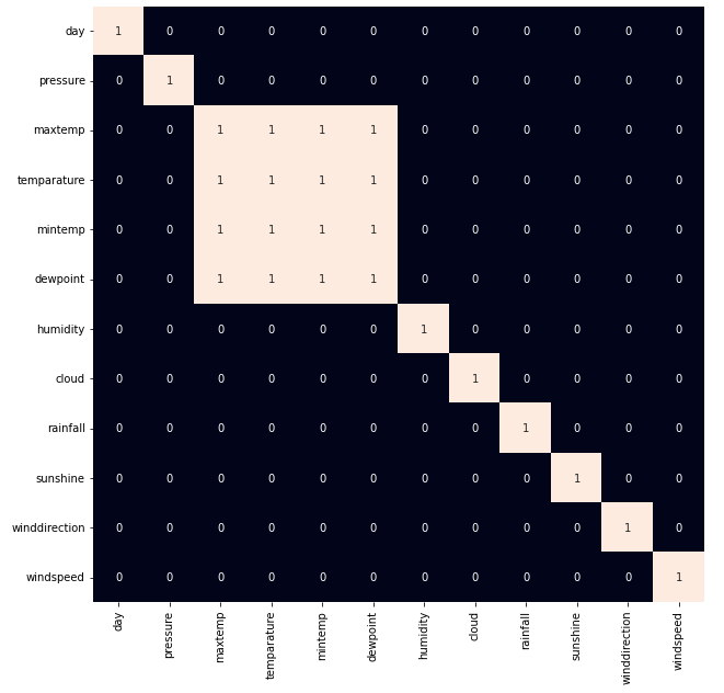 现在我们将删除高度相关的特征’maxtemp’和’mintep’。但为什么不是temp或dewpoint呢?这是因为temp和dewpoint提供了关于天气和大气条件的不同信息。
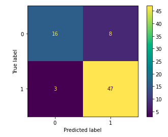 让我们使用SVC模型绘制验证数据的分类报告。
【本文地址】
今日新闻 |
推荐新闻 |