无人驾驶算法 |
您所在的位置:网站首页 › 自动驾驶路径规划与轨迹跟踪的区别 › 无人驾驶算法 |
无人驾驶算法
|
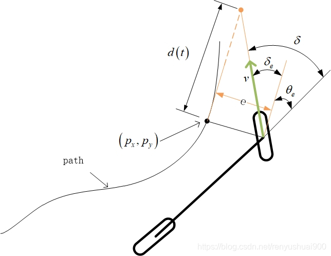
一、基于几何追踪的方法 关于无人车追踪轨迹,目前的主流方法分为两类:基于几何追踪的方法和基于模型预测的方法,其中几何追踪方法主要包含纯跟踪和Stanley两种方法,纯跟踪方法已经广泛应用于移动机器人的路径跟踪中,网上也有很多详细的介绍,本文主要介绍斯坦福大学无人车使用的Stanley方法。
上面的state.yaw根据当前车辆方向盘转角控制量delta跟速度v、半径长度L得到当前车辆在dt时间转过的角度,即,新增的航向角。 def PControl(target, current): a = Kp * (target - current) return a def stanley_control(state, cx, cy, ch, pind): ind = calc_target_index(state, cx, cy) if pind >= ind: ind = pind if ind < len(cx): tx = cx[ind] ty = cy[ind] th = ch[ind] else: tx = cx[-1] ty = cy[-1] th = ch[-1] ind = len(cx) - 1 # 计算横向误差 if ((state.x - tx) * th - (state.y - ty)) > 0: error = abs(math.sqrt((state.x - tx) ** 2 + (state.y - ty) ** 2)) else: error = -abs(math.sqrt((state.x - tx) ** 2 + (state.y - ty) ** 2)) #此路线节点期望的航向角减去当前车辆航向角(航向偏差),然后再加上横向偏差角即match.atan()得到的值 #得到的delta即为控制车辆方向盘的控制量 delta = ch[ind] - state.yaw + math.atan2(k * error, state.v) # 限制车轮转角 [-30, 30] if delta > np.pi / 6.0: delta = np.pi / 6.0 elif delta < - np.pi / 6.0: delta = - np.pi / 6.0 return delta, ind定义函数用于搜索最临近的路点: def calc_target_index(state, cx, cy): # 搜索最临近的路点 dx = [state.x - icx for icx in cx] dy = [state.y - icy for icy in cy] d = [abs(math.sqrt(idx ** 2 + idy ** 2)) for (idx, idy) in zip(dx, dy)] ind = d.index(min(d)) return ind主函数: def main(): # 设置目标路点 cx = np.arange(0, 50, 1) cy = [0 * ix for ix in cx] #路径的结点处的航向角,指的是车身整体 ch = [0 * ix for ix in cx] target_speed = 5.0 / 3.6 # [m/s] T = 200.0 # 最大模拟时间 # 设置车辆的初始状态 state = VehicleState(x=-0.0, y=-3.0, yaw=-0.0, v=0.0) lastIndex = len(cx) - 1 time = 0.0 x = [state.x] y = [state.y] #当前车身的航向角 yaw = [state.yaw] v = [state.v] t = [0.0] target_ind = calc_target_index(state, cx, cy) while T >= time and lastIndex > target_ind: ai = PControl(target_speed, state.v) di, target_ind = stanley_control(state, cx, cy, ch, target_ind) state = update(state, ai, di) time = time + dt x.append(state.x) y.append(state.y) yaw.append(state.yaw) v.append(state.v) t.append(time) plt.cla() plt.plot(cx, cy, ".r", label="course") plt.plot(x, y, "-b", label="trajectory") plt.plot(cx[target_ind], cy[target_ind], "go", label="target") plt.axis("equal") plt.grid(True) plt.title("Speed[km/h]:" + str(state.v * 3.6)[:4]) plt.pause(0.001) if __name__ == '__main__': main()仿真结果:
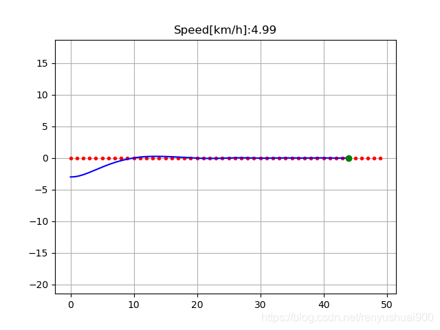
通过仿真结果图,我们看到红点表示实现规划好的直线路径,蓝线则表示我们的车辆实际运行的轨迹,绿点表示距离当前位置最近路径点,在这段代码中,我们设置了增益参数kkk为0.3,通过进一步去改变kkk的大小对比结果,可以减小kkk值得到更平滑的跟踪轨迹,但是更加平滑的结果会引起某些急剧的转角处会存在转向不足的情况。 参考 Automatic Steering Methods for Autonomous Automobile Path TrackingStanley_ The robot that won the DARPA grand challenge无人驾驶汽车系统入门(十八)——使用pure pursuit实现无人车轨迹追踪(https://blog.csdn.net/adamshan/article/details/80555174)无人驾驶算法——使用Stanley method实现无人车轨迹追踪 |


【本文地址】