ERA5数据下载和批处理教程 |
您所在的位置:网站首页 › 气象数据下载免费软件 › ERA5数据下载和批处理教程 |
ERA5数据下载和批处理教程
|
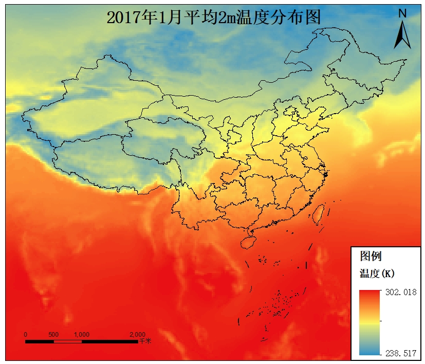
ERA5 再分析数据是最新一代的再分析数据,由欧盟资助的哥白尼气候变化服务(C3S)创建,由 ECMWF 运营。同化了包括全球范围内不同区域和来源的遥感资料、地表与上层大气常规气象资料。它覆盖了 1950 年至今的历史时期,实现了实时更新,延迟约 3 个月。ERA5 在其前身 ERA-Interim 的基础上进行了大幅升级,在时间分辨率和空间分辨率上都有显著提高。 ERA5 再分析资料提供了许多种类的要素,包括 2m 温度、2m 相对湿度、海平面气压、10m 风等地面要素以及温度、相对湿度、位势高度、风场等高空要素。 ⛄ERA5数据下载本例子以ERA5 monthly averaged data on single levels from 1959 to present数据为基础,下载2017、2018、2019、2020、2021年ERA5再分析数据,并进行批处理。数据变量主要包括: 2m_temperatureskin_temperaturetotal_precipitation 👀前期准备进入 Climate Data Store(CDS),官方网站,注册新用户(已有请忽略) 选择需要的数据,以ERA5 monthly averaged data on single levels from 1959 to present数据为例,在Download data选项卡里面产品类型Product type和变量Variable选择对应的Year、Month、Time;地理区域Geographical area;格式Format为NetCDF;Terms of use 勾上对号Licence to use Copernicus Products;最下面有三种下载方式①Show API request;②Show Toolbox request;③Submit Form。 👀Python方式下载点击Show API request,出现Python代码,是根据你选择的数据自动生成的API请求。 import cdsapi c = cdsapi.Client() c.retrieve( 'reanalysis-era5-single-levels-monthly-means', { 'product_type': 'monthly_averaged_reanalysis', 'variable': [ '2m_temperature', 'skin_temperature', 'total_precipitation', ], 'year': [ '2017', '2018', '2019', '2020', '2021', ], 'month': [ '01', '02', '03', '04', '05', '06', '07', '08', '09', '10', '11', '12', ], 'time': '00:00', 'area': [ 60, 70, 0, 140, ], 'format': 'netcdf', }, 'download.nc')运行成功此代码,需要以下准备: (1)安装cdsapi模块 pip install cdsapi(2)此时可能运行出错 Exception: Missing/incomplete configuration file:C:\Users\Administrator/.cdsapirc初步分析:在目标路径下缺少.cdsapirc文件,该文件里含有下载数据的url和key 解决方案:针对已注册的用户,进入How to use the CDS API网站,获得url和key url: https://cds.climate.copernicus.eu/api/v2 key: *****************************************(已隐藏) 新建txt文件,将自己的url和key复制进去,然后保存;把txt文件名改为.cdsapirc(注意有.),同时修改文件后缀名,即把.txt后缀删除;将文件复制或剪切到之前报错的目标路径下;运行Python程序,即可成功下载。 👀IDM下载器方式下载点击Submit Form,跳转界面到Your requests,会显示当前下载数据的请求状态,需要你耐心等待一会儿。 通过请求之后,即可通过Internet Download Manager(IDM)下载器下载(前提已安装)。 ⛄ERA5数据批处理ERA5数据批处理目标要求: 读取nc文件;查看并获取nc文件中对应变量的信息;根据数据的经纬度,计算分辨率;定义投影;保存数据为tif格式。 👀流程步骤(1)读取nc文件 安装对应的netCDF4模块 pip install netCDF4 import netCDF4 as nc # 读取nc文件 tep_data = nc.Dataset(input_path)(2)查看并获取nc文件中对应变量的信息 # 查看nc文件中的变量信息 print(tep_data.variables.keys()) # 获取nc文件中对应变量的信息 lon_data = tep_data.variables["longitude"][:] lat_data = tep_data.variables["latitude"][:](3)根据数据的经纬度,计算分辨率 # 影像的左上角&右下角坐标 lonmin, latmax, lonmax, latmin = [lon_data.min(), lat_data.max(), lon_data.max(), lat_data.min()] # print(lonmin, latmax, lonmax, latmin) # 分辨率计算 num_lon = len(lon_data) num_lat = len(lat_data) lon_res = (lonmax - lonmin) / (float(num_lon) - 1) lat_res = (latmax - latmin) / (float(num_lat) - 1) print(num_lon, num_lat) print(lon_res, lat_res)(4)定义投影 # 定义投影 proj = osr.SpatialReference() proj.ImportFromEPSG(4326) # WGS84 proj = proj.ExportToWkt() # 重点,转成wkt格式 # print(prj) 字符串 # 定义六参数,设置影像的显示范围和分辨率 # 影像左上角横坐标:geoTransform[0] # 影像左上角纵坐标:geoTransform[3] # 遥感图像的水平空间分辨率为geoTransform[1] # 遥感图像的垂直空间分辨率为geoTransform[5] # 通常geoTransform[5] 与 geoTransform[1]相等 # 如果遥感影像方向没有发生旋转,即上北、下南,则geoTransform[2] 与 row *geoTransform[4] 为零。 geotransform = (lonmin, lon_res, 0.0, latmax, 0.0, -lat_res)(5)保存数据为tif格式,以2m_temperature(t2m)温度为例 t2m = tep_data.variables["t2m"][:] # 用np.array把数据转化成数组(矩阵)类型 t2m_arr = np.asarray(t2m) #年份 yearlist = [2017,2018,2019,2020,2021] for i in range(len(yearlist)): year = yearlist[i] for j in range(12*i, 12*(i+1)): month = (j % 12) + 1 outputpath = output_path + str(year) + "_" + str(month) + "_t2m.tif" write_img(outputpath, proj, geotransform, t2m_arr[j]) 👀结果文件展示 2017_1_t2m.tif 2017_2_t2m.tif 2017_3_t2m.tif 2017_4_t2m.tif 2017_5_t2m.tif 2017_6_t2m.tif ... ... 2021_7_t2m.tif 2021_8_t2m.tif 2021_9_t2m.tif 2021_10_t2m.tif 2021_11_t2m.tif 2021_12_t2m.tif以2017_1_t2m.tif结果为例,如下图:
笔者不才,多多交流!!! 欢迎大家关注预览我的博客Blog:HeartLoveLife 能力有限,敬请谅解!! |
【本文地址】
今日新闻 |
推荐新闻 |