利用MATLAB绘制极坐标等值线图 |
您所在的位置:网站首页 › 极坐标绘图用什么函数表示 › 利用MATLAB绘制极坐标等值线图 |
利用MATLAB绘制极坐标等值线图
|
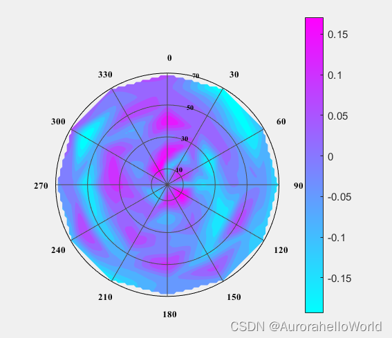
ContourPolor函数是MathWorks公司在1984年开发的绘图函数,主要用于解决MATLAB中极坐标等值线图的绘制问题。 什么是极坐标等值线图? 网上没有明确的概念,先放一张画好的图让大家直观地感受一下,下面这个就是极坐标等值线图:
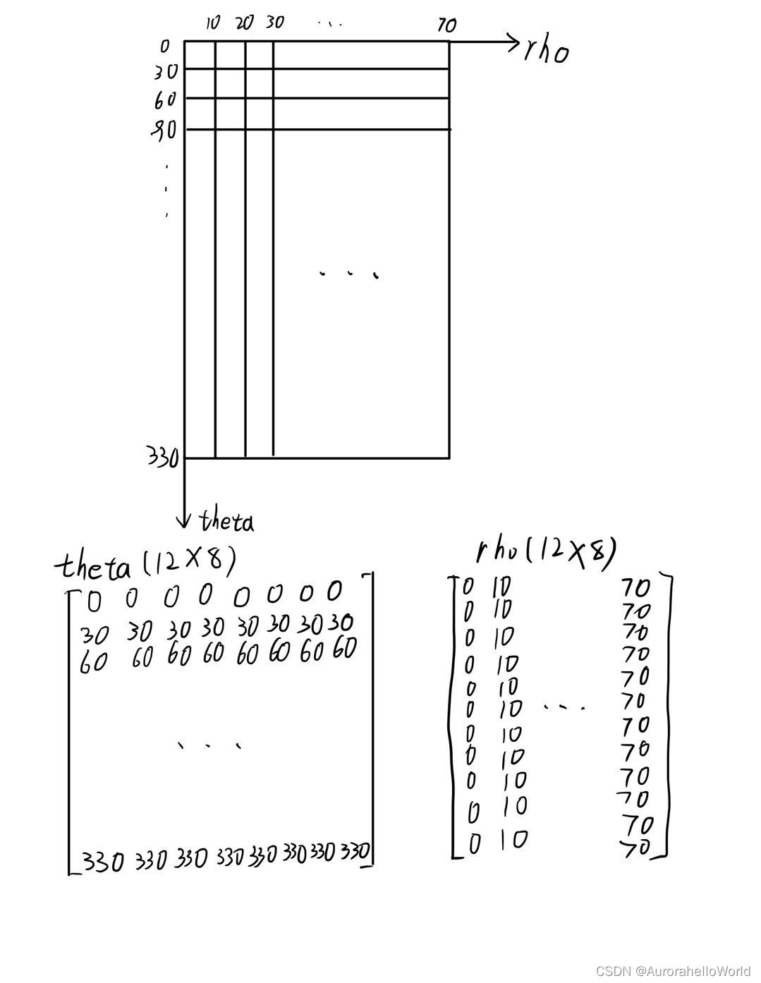
看着上面的图,我们可以更深入地理解一下它的名字:首先,它的坐标系为极坐标,即每一个方位角,每一个半径都对应一个属性数值;其次,它的图面是由每一个散点的空间位置和属性数值进行内插得到的一圈圈等值线组成的。 那有的小伙伴就会问了,这个图有什么用,能干什么? 在笔者研究的遥感领域,对于BRDF(双向反射分布函数)可以反应地物反射率的各向异性,对于反射率方向性分布的研究也是定量遥感中重要的研究领域和方向,而假如利用平面的方位角表示观测或入射的方位角、利用不同的圆圈表示半球空间中的天顶角,极坐标等值线图可以极好地刻画半球空间中的一些属性,且形式直观易懂,理解方便,对于以上方面的研究分析有着至关重要的作用,也是期刊论文插图中常见的形式;另外,在其他领域,如流体力学、地球物理等学科,但凡需要分析半球空间上的属性差异,都可以采用极坐标等值线图。 这么重要的图,还不快快学起来,用到期刊论文插图里泰裤辣!!! 笔者结合几天的学习成果和代码(Copyright (c) 1984-98 by The MathWorks, Inc.引用代码为了解释和传播知识,如有侵权请联系笔者删除)为大家详细讲解一下MATLAB实现代码: 1.输入参数处理这部分主要是对输入参数多样性进行处理,利用MATLAB可变参数和条件语句的原理(不懂的小伙伴可以搜一下)对输入参数的各种情况进行判断和处理,以避免错误的输入。 划重点了:我们知道,一个半球空间中任意一条通过球心向外的直线和其与球面交点的位置可以通过方位角和天顶角来唯一确定,而这个函数的输入可以理解为一个二维曲面函数,由一个个平面数对和数对对应的属性值组成,每一个数对为一个方位角theta和天顶角rho,而其对应球面位置的属性值则为z,即(theta,rho)——>z,这也就相当于二元函数中的平面坐标(x,y)和其对应的值z,而输入参数theta则为(theta,rho)数对中theta的值矩阵,theta则为(theta,rho)数对中rho的值矩阵,z则为对应的属性值矩阵,所以theta、rho、z矩阵的大小应该完全相同,如果还不理解,请看下图,我们就分析一下上面的那张极坐标等值线图的输入参数:
口说无凭,太抽象,不好理解,结合这张图,我们就可以更好地理解theta、rho矩阵的含义了,相当于把一个平面每一个格网点的坐标拆解成x和y两个矩阵,还是不明白的可以查看meshgrid函数的帮助文档(命令行窗口中输入help meshgrid),更好地理解一下这个坐标格网的分解关系。当然,这两个矩阵可以用MATLAB自带的ndgrid函数生成(不了解的小伙伴可以在MATLAB命令行窗口中输入help ndgrid查看帮助文档),然后注意z值要与坐标格网中的(theta,rho)数对一一对应。 而参数n则是想要生成等值线的条数,maxrho为rho的最大值。 function hpol = ContourPolar(theta,rho,z,n,maxrho) %ContourPolar Polar coordinate plot. %这个函数可以绘制极坐标等值线图 % modified from POLAR in 2001/01/01 % Copyright (c) 1984-98 by The MathWorks, Inc. % $Revision: 5.17 $ $Date: 1998/09/30 15:25:05 $ %theta 观测方位角 %rho 观测天顶角 %z 反射率值 %n 等值线的条数 %maho 极径的最大值 %输入参数中方位角和天顶角组合成数对,每个数对x坐标为方位角,y坐标为天顶角,theta为数对的x坐标,rho为数对的y坐标,z为每个数对对应的数值 d = 0.5; % axes('Parent',gcf,'position',[0.10 0.10 0.5 0.5]); maxvza = maxrho; if nargin < 4%输入三个参数,默认等值线8条 n = 8; end if nargin < 5%输入四个参数,默认maxrho = max(rho) maxrho = max(rho); end if isstr(theta) | isstr(rho) error('Input arguments must be numeric.'); end if ~isequal(size(theta),size(rho)) error('THETA and RHO must be the same size.'); end 2.生成极坐标等值线图的内核好了,弄懂了输入参数,我们看接下来的画图部分,下面这个代码就是生成极坐标等值线图的核心代码,这一段其实不需要我们修改什么参数,我们只需要知道绘图原理即可,就是首先通过坐标转换将(theta,rho,z)值放到图面相应的位置上去,接着生成格网,进行曲面拟合,拟合出二次曲面后根据曲面绘制等值线: % get hold state cax = newplot; next = lower(get(cax,'NextPlot'));%结果'replace' hold_state = ishold;%获取当前hold状态 % transform data to Cartesian coordinates.(笛卡尔坐标) delta = maxrho/50; xx = rho.*cos((90-theta)*(pi/180)); yy = rho.*sin((90-theta)*(pi/180)); xi = -maxrho:delta:maxrho; yi = xi; [xi,yi] = meshgrid(xi,yi); zi = griddata(xx,yy,z,xi,yi,'cubic'); [M,c] = contourf(xi,yi,zi,n); % c.LineStyle = '-'; c.LineStyle = 'none'; c.LineWidth = d; % c.LineColor = 'w'; % c.LineWidth = 0.000000000000000000000001; %surf(xi,yi,zi); % axis([-60,60,-60,60,25,40]); %view(0,90); %shading flat; % get x-axis text color so grid is in same color tc = get(cax,'xcolor'); ls = get(cax,'gridlinestyle'); % Hold on to current Text defaults, reset them to the % Axes' font attributes so tick marks use them. fAngle = get(cax, 'DefaultTextFontAngle'); fName = get(cax, 'DefaultTextFontName'); fSize = get(cax, 'DefaultTextFontSize'); fWeight = get(cax, 'DefaultTextFontWeight'); fUnits = get(cax, 'DefaultTextUnits'); % set(cax, 'DefaultTextFontAngle', get(cax, 'FontAngle'), ... % 'DefaultTextFontName', get(cax, 'FontName'), ... % 'DefaultTextFontSize', get(cax, 'FontSize'), ... % 'DefaultTextFontWeight', get(cax, 'FontWeight'), ... % 'DefaultTextUnits','data') % only do grids if hold is off if ~hold_state % make a radial grid hold on; maxrho = max(abs(rho(:))); hhh=plot([-maxrho -maxrho maxrho maxrho],[-maxrho maxrho maxrho -maxrho],'linewidth',d); set(gca,'dataaspectratio',[1 1 1],'plotboxaspectratiomode','auto') v = [get(cax,'xlim') get(cax,'ylim')]; ticks = sum(get(cax,'ytick')>=0); delete(hhh); % check radial limits and ticks rmin = 0; rmax = v(4); rticks = max(ticks-1,2); if rticks > 5 % see if we can reduce the number if rem(rticks,2) == 0 rticks = rticks/2; elseif rem(rticks,3) == 0 rticks = rticks/3; end end 3.生成外侧同心圆接下来这一段代码就是绘制我们在图上看到的外侧的一个个同心圆,我们可以修改for i=(rmin+rinc):2*rinc:maxvza,控制同心圆数量和显示的位置,向量中每一个值就是同心圆显示的位置,比如,我画的那张这里i的值就是10:20:70,这里rmin默认是0,rinc默认是10,可以根据需要自行修改。 % define a circle th = 0:pi/50:2*pi; xunit = cos(th); yunit = sin(th); % now really force points on x/y axes to lie on them exactly inds = 1:(length(th)-1)/4:length(th); xunit(inds(2:2:4)) = zeros(2,1); yunit(inds(1:2:5)) = zeros(3,1); % plot background if necessary % if ~isstr(get(cax,'color')), % patch('xdata',xunit*rmax,'ydata',yunit*rmax, ... % 'edgecolor',tc,'facecolor',get(gca,'color'),... % 'handlevisibility','off'); % end % draw radial circles c82 = cos(80*pi/180); s82 = sin(80*pi/180); % rinc = (rmax-rmin)/6;%rticks; 天顶角圆圈个数 % for i=(rmin+rinc):rinc:rmax % hhh = plot(xunit*i,yunit*i,ls,'color',tc,'linewidth',1,... % 'handlevisibility','off'); % % end % set(hhh,'linestyle','-') % Make outer circle solid % for i=(rmin):2*rinc:rmax % % text((i+rinc/20)*c82,(i+rinc/20)*s82, ... % [' \fontsize{15} ' num2str(i)],'verticalalignment','bottom',... % 'handlevisibility','off','Color','r') % end rinc = 10;%(rmax-rmin)/6;%rticks; 天顶角圆圈个数,画径向圆圈%%%%%%%%%%%%%%%%%%%%%%%%%%%%%%%%%%%%%%% for i=(rmin+rinc):2*rinc:maxvza%可以根据输入的rho修改这里,控制同心圆数量和显示的位置 hhh = plot(xunit*i,yunit*i,'-','color',[.3,0.3 0.3],'linewidth',d,... 'handlevisibility','off'); end hhh = plot(xunit*maxvza,yunit*maxvza,'-','color',[0 0 0],'linewidth',d,... 'handlevisibility','off'); set(hhh,'linestyle','-') % Make outer circle solid 4.标注天顶角接下来这一段代码是控制天顶角的标注,可以根据需要对i向量的值进行调整,i的值就是显示在图上的天顶角值,比如,我画的图里i的值为20:20:80,另外,fontsize为字号大小,fontname为字体,verticalalignment为标注在线上的位置,有up,middle,bottom三种位置,可以根据需要自己调整然后试一下,从而选择合适的字体、字号和位置。 %标注刻度 for i=20:20:80 text((i-10+rinc/20)*c82,(i-10+rinc/20)*s82, ... [' \fontsize{6} ' num2str(i-10)],'verticalalignment','middle',... 'handlevisibility','off','fontname','times new roman','fontweight','bold') end % text((75-10+rinc/20)*c82,(75-10+rinc/20)*s82, ... % [' \fontsize{10} ' num2str(75)],'verticalalignment','bottom',... % 'handlevisibility','off')%,'Color','r' 5.标注方位角和轴至于方位角和轴的标注,我们也不用改,保持默认就行,这一块我也没有研究,如果有小伙伴研究了修改方法欢迎在评论区交流补充,下面是标注方位角和轴的代码: % plot spokes th = (1:6)*2*pi/12; cst = cos(pi/2-th); snt = sin(pi/2-th); cs = [-cst; cst]; sn = [-snt; snt]; plot(rmax*cs,rmax*sn,'-','color',[.3,0.3 0.3],'linewidth',d,... 'handlevisibility','off') % annotate spokes in degrees rt = 1.15*rmax; for i = 1:1:length(th)%%%%%%%%%%%%%%%%%%%%%%%%%%%%%%%%%%%%%%%%%%%%%%%%%%%%%%%%%%%%%%%% text(rt*cst(i),rt*snt(i),[' \fontsize{8} ' int2str(i*30)],'horizontalalignment','center','handlevisibility','off','fontname','times new roman','fontweight','bold'); if i == length(th) loc = int2str(0); else loc = int2str(180+i*30); end text(-rt*cst(i),-rt*snt(i), [' \fontsize{8} ' loc],'horizontalalignment','center',... 'handlevisibility','off','fontname','times new roman','fontweight','bold') end % set view to 2-D view(2); % set axis limits axis(rmax*[-1.15 1.15 -1.15 1.5]);%%%%%%%%%%%%%%%%%%%%%%%%%%%%%%%%%%%%%%%%%%%%%%%%%%%%%%%%%%%%%%%% end % Reset defaults. set(cax, 'DefaultTextFontAngle', fAngle , ... 'DefaultTextFontName', fName , ... 'DefaultTextFontSize', fSize, ... 'DefaultTextFontWeight', fWeight, ... 'DefaultTextUnits',fUnits ); % plot data on top of grid if nargout > 0 hpol = q; end if ~hold_state set(gca,'dataaspectratio',[1 1 1]), axis off; set(cax,'NextPlot',next); end set(get(gca,'xlabel'),'visible','on'); set(get(gca,'ylabel'),'visible','on'); %colormap gray; %pcolor(255,255,255); colormap cool; end补充一句,上面这段代码可以修改极坐标等值线图的色带,通过修改colormap后面的属性进行,MATLAB色带可以通过这篇文章查看https://blog.csdn.net/sinat_21026543/article/details/80215281?spm=1001.2014.3001.5506 也可以自己多换几种色带试一试。 另外,要插入颜色带,可以使用加入colorbar(可以搜索帮助文档help colorbar进行查看),并通过设置对象进行颜色带属性修改。 到这里,这个函数就讲解完了,下面是ContourPolor函数的完整代码,版权属于MathWorks公司,这里只是转载,有需要的小伙伴可以自行取用并根据上面的讲解修改参数: function hpol = ContourPolar(theta,rho,z,n,maxrho) %ContourPolar Polar coordinate plot. %这个函数可以绘制极坐标等值线图 % modified from POLAR in 2001/01/01 % Copyright (c) 1984-98 by The MathWorks, Inc. % $Revision: 5.17 $ $Date: 1998/09/30 15:25:05 $ %theta 观测方位角 %rho 观测天顶角 %z 反射率值 %n 等值线的条数 %maho 极径的最大值 %输入参数中方位角和天顶角组合成数对,每个数对x坐标为方位角,y坐标为天顶角,theta为数对的x坐标,rho为数对的y坐标,z为每个数对对应的数值 d = 0.5; % axes('Parent',gcf,'position',[0.10 0.10 0.5 0.5]); maxvza = maxrho; if nargin < 4%输入三个参数,默认等值线8条 n = 8; end if nargin < 5%输入四个参数,默认maxrho = max(rho) maxrho = max(rho); end if isstr(theta) | isstr(rho) error('Input arguments must be numeric.'); end if ~isequal(size(theta),size(rho)) error('THETA and RHO must be the same size.'); end % get hold state cax = newplot; next = lower(get(cax,'NextPlot'));%结果'replace' hold_state = ishold;%获取当前hold状态 % transform data to Cartesian coordinates.(笛卡尔坐标) delta = maxrho/50; xx = rho.*cos((90-theta)*(pi/180)); yy = rho.*sin((90-theta)*(pi/180)); xi = -maxrho:delta:maxrho; yi = xi; [xi,yi] = meshgrid(xi,yi); zi = griddata(xx,yy,z,xi,yi,'cubic'); [M,c] = contourf(xi,yi,zi,n); % c.LineStyle = '-'; c.LineStyle = 'none'; c.LineWidth = d; % c.LineColor = 'w'; % c.LineWidth = 0.000000000000000000000001; %surf(xi,yi,zi); % axis([-60,60,-60,60,25,40]); %view(0,90); %shading flat; % get x-axis text color so grid is in same color tc = get(cax,'xcolor'); ls = get(cax,'gridlinestyle'); % Hold on to current Text defaults, reset them to the % Axes' font attributes so tick marks use them. fAngle = get(cax, 'DefaultTextFontAngle'); fName = get(cax, 'DefaultTextFontName'); fSize = get(cax, 'DefaultTextFontSize'); fWeight = get(cax, 'DefaultTextFontWeight'); fUnits = get(cax, 'DefaultTextUnits'); % set(cax, 'DefaultTextFontAngle', get(cax, 'FontAngle'), ... % 'DefaultTextFontName', get(cax, 'FontName'), ... % 'DefaultTextFontSize', get(cax, 'FontSize'), ... % 'DefaultTextFontWeight', get(cax, 'FontWeight'), ... % 'DefaultTextUnits','data') % only do grids if hold is off if ~hold_state % make a radial grid hold on; maxrho = max(abs(rho(:))); hhh=plot([-maxrho -maxrho maxrho maxrho],[-maxrho maxrho maxrho -maxrho],'linewidth',d); set(gca,'dataaspectratio',[1 1 1],'plotboxaspectratiomode','auto') v = [get(cax,'xlim') get(cax,'ylim')]; ticks = sum(get(cax,'ytick')>=0); delete(hhh); % check radial limits and ticks rmin = 0; rmax = v(4); rticks = max(ticks-1,2); if rticks > 5 % see if we can reduce the number if rem(rticks,2) == 0 rticks = rticks/2; elseif rem(rticks,3) == 0 rticks = rticks/3; end end % define a circle th = 0:pi/50:2*pi; xunit = cos(th); yunit = sin(th); % now really force points on x/y axes to lie on them exactly inds = 1:(length(th)-1)/4:length(th); xunit(inds(2:2:4)) = zeros(2,1); yunit(inds(1:2:5)) = zeros(3,1); % plot background if necessary % if ~isstr(get(cax,'color')), % patch('xdata',xunit*rmax,'ydata',yunit*rmax, ... % 'edgecolor',tc,'facecolor',get(gca,'color'),... % 'handlevisibility','off'); % end % draw radial circles c82 = cos(80*pi/180); s82 = sin(80*pi/180); % rinc = (rmax-rmin)/6;%rticks; 天顶角圆圈个数 % for i=(rmin+rinc):rinc:rmax % hhh = plot(xunit*i,yunit*i,ls,'color',tc,'linewidth',1,... % 'handlevisibility','off'); % % end % set(hhh,'linestyle','-') % Make outer circle solid % for i=(rmin):2*rinc:rmax % % text((i+rinc/20)*c82,(i+rinc/20)*s82, ... % [' \fontsize{15} ' num2str(i)],'verticalalignment','bottom',... % 'handlevisibility','off','Color','r') % end rinc = 10;%(rmax-rmin)/6;%rticks; 天顶角圆圈个数,画径向圆圈%%%%%%%%%%%%%%%%%%%%%%%%%%%%%%%%%%%%%%% for i=(rmin+rinc):2*rinc:maxvza hhh = plot(xunit*i,yunit*i,'-','color',[.3,0.3 0.3],'linewidth',d,... 'handlevisibility','off'); end hhh = plot(xunit*maxvza,yunit*maxvza,'-','color',[0 0 0],'linewidth',d,... 'handlevisibility','off'); set(hhh,'linestyle','-') % Make outer circle solid %标注刻度 for i=20:20:80 text((i-10+rinc/20)*c82,(i-10+rinc/20)*s82, ... [' \fontsize{6} ' num2str(i-10)],'verticalalignment','middle',... 'handlevisibility','off','fontname','times new roman','fontweight','bold') end % text((75-10+rinc/20)*c82,(75-10+rinc/20)*s82, ... % [' \fontsize{10} ' num2str(75)],'verticalalignment','bottom',... % 'handlevisibility','off')%,'Color','r' % plot spokes th = (1:6)*2*pi/12; cst = cos(pi/2-th); snt = sin(pi/2-th); cs = [-cst; cst]; sn = [-snt; snt]; plot(rmax*cs,rmax*sn,'-','color',[.3,0.3 0.3],'linewidth',d,... 'handlevisibility','off') % annotate spokes in degrees rt = 1.15*rmax; for i = 1:1:length(th)%%%%%%%%%%%%%%%%%%%%%%%%%%%%%%%%%%%%%%%%%%%%%%%%%%%%%%%%%%%%%%%% text(rt*cst(i),rt*snt(i),[' \fontsize{8} ' int2str(i*30)],'horizontalalignment','center','handlevisibility','off','fontname','times new roman','fontweight','bold'); if i == length(th) loc = int2str(0); else loc = int2str(180+i*30); end text(-rt*cst(i),-rt*snt(i), [' \fontsize{8} ' loc],'horizontalalignment','center',... 'handlevisibility','off','fontname','times new roman','fontweight','bold') end % set view to 2-D view(2); % set axis limits axis(rmax*[-1.15 1.15 -1.15 1.5]);%%%%%%%%%%%%%%%%%%%%%%%%%%%%%%%%%%%%%%%%%%%%%%%%%%%%%%%%%%%%%%%% end % Reset defaults. set(cax, 'DefaultTextFontAngle', fAngle , ... 'DefaultTextFontName', fName , ... 'DefaultTextFontSize', fSize, ... 'DefaultTextFontWeight', fWeight, ... 'DefaultTextUnits',fUnits ); % plot data on top of grid if nargout > 0 hpol = q; end if ~hold_state set(gca,'dataaspectratio',[1 1 1]), axis off; set(cax,'NextPlot',next); end set(get(gca,'xlabel'),'visible','on'); set(get(gca,'ylabel'),'visible','on'); %colormap gray; %pcolor(255,255,255); colormap cool; end我还上传了ContourPolor函数的代码包,也可以下载代码包,为MATLAB的.m文件。 再次声明一下:ContourPolor函数是MathWorks公司在1984年开发的绘图函数,本文的内容和代码包只是转载和传播知识,如涉及侵权请联系笔者删除文章。 如果您觉得文章内容对您有帮助,欢迎点赞收藏,也欢迎关注笔者,您的支持是我继续发布优质文章,分析优质资源的巨大动力。另外,文章如有错误之处欢迎在评论区批评指正,如果有疑惑也欢迎大家在评论区留言讨论,笔者会一一解答。 |
【本文地址】