GEE:LandTrendr时间序列曲线拟合 |
您所在的位置:网站首页 › 时间序列预测怎么看拟合测量的结果 › GEE:LandTrendr时间序列曲线拟合 |
GEE:LandTrendr时间序列曲线拟合
|
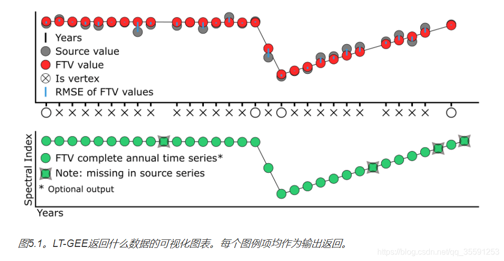
毕竟是时间序列分析,LandTrendr的时间序列曲线是怎么拟合的?在一个像素点的位置上,它是怎么输出变化年份、扰动幅度、恢复幅度和时间的? 以下代码给出了回答,可以参考LT-GEE官方的说明文档。 用LandTrendr选取指定像素点的APP:https://emaprlab.users.earthengine.app/view/lt-gee-pixel-time-series LT-GEE的结果包括: 每个像素时间序列的观测年份;二维频谱时间空间中的x轴值;(默认) 每个像素时间序列的观测值的源值;二维频谱时间空间中的y轴值;(默认) 拟合到每个像素时间序列的顶点之间的线段(FTV)的观测值的源值;二维频谱时间空间中的y轴值;(默认) FTV值相对于源值的均方根误差(RMSE);(默认) 集合中大于波段1的其他波段的完整时间序列FTV值;二维频谱时间空间中的y轴值;(可选的) 时间序列曲线拟合,结果如下图所示: 源代码:(复制粘贴到GEE里面就可以直接运行了)https://code.earthengine.google.com/12a8d012f2a566995a7c1de1c257b479?noload=true //# LANDTRENDR SOURCE AND FITTING PIXEL TIME SERIES // date: 2018-04-19 // author: Zhiqiang Yang | [email protected] // Justin Braaten | [email protected] // Robert Kennedy | [email protected] // website: https://github.com/eMapR/LT-GEE // 首先输入一个点的经纬度 var long = -122.8848; var lat = 43.7929; // 定义数据集参数 var startYear = 1985; // 时间序列开始年份 var endYear = 2017; // 时间序列结束年份 var startDay = '06-01'; // 筛选每年的开始时间 var endDay = '09-30'; // 筛选每年的结束时间 // 计算光谱指数(NDVI等) var segIndex = function(img) { var index = img.normalizedDifference(['B4', 'B7']) .multiply(1000) .select([0], ['NBR']) .set('system:time_start', img.get('system:time_start')); return index ; }; var distDir = -1; // define the sign of spectral delta for vegetation loss for the segmentation index - // NBR delta is negetive for vegetation loss, so -1 for NBR, 1 for band 5, -1 for NDVI, etc // define the segmentation parameters: // reference: Kennedy, R. E., Yang, Z., & Cohen, W. B. (2010). Detecting trends in forest disturbance and recovery using yearly Landsat time series: 1. LandTrendr—Temporal segmentation algorithms. Remote Sensing of Environment, 114(12), 2897-2910. // https://github.com/eMapR/LT-GEE var run_params = { maxSegments: 6, spikeThreshold: 0.9, vertexCountOvershoot: 3, preventOneYearRecovery: true, recoveryThreshold: 0.25, pvalThreshold: 0.05, bestModelProportion: 0.75, minObservationsNeeded: 6 }; //################################################################################################ //######################################################################################################## //##### ANNUAL SR TIME SERIES COLLECTION BUILDING FUNCTIONS ##### //######################################################################################################## //----- MAKE A DUMMY COLLECTOIN FOR FILLTING MISSING YEARS ----- var dummyCollection = ee.ImageCollection([ee.Image([0,0,0,0,0,0]).mask(ee.Image(0))]); // make an image collection from an image with 6 bands all set to 0 and then make them masked values //------ L8 to L7 HARMONIZATION FUNCTION ----- // slope and intercept citation: Roy, D.P., Kovalskyy, V., Zhang, H.K., Vermote, E.F., Yan, L., Kumar, S.S, Egorov, A., 2016, Characterization of Landsat-7 to Landsat-8 reflective wavelength and normalized difference vegetation index continuity, Remote Sensing of Environment, 185, 57-70.(http://dx.doi.org/10.1016/j.rse.2015.12.024); Table 2 - reduced major axis (RMA) regression coefficients var harmonizationRoy = function(oli) { var slopes = ee.Image.constant([0.9785, 0.9542, 0.9825, 1.0073, 1.0171, 0.9949]); // create an image of slopes per band for L8 TO L7 regression line - David Roy var itcp = ee.Image.constant([-0.0095, -0.0016, -0.0022, -0.0021, -0.0030, 0.0029]); // create an image of y-intercepts per band for L8 TO L7 regression line - David Roy var y = oli.select(['B2','B3','B4','B5','B6','B7'],['B1', 'B2', 'B3', 'B4', 'B5', 'B7']) // select OLI bands 2-7 and rename them to match L7 band names .resample('bicubic') // ...resample the L8 bands using bicubic .subtract(itcp.multiply(10000)).divide(slopes) // ...multiply the y-intercept bands by 10000 to match the scale of the L7 bands then apply the line equation - subtract the intercept and divide by the slope .set('system:time_start', oli.get('system:time_start')); // ...set the output system:time_start metadata to the input image time_start otherwise it is null return y.toShort(); // return the image as short to match the type of the other data }; //------ RETRIEVE A SENSOR SR COLLECTION FUNCTION ----- var getSRcollection = function(year, startDay, endDay, sensor, aoi) { // get a landsat collection for given year, day range, and sensor var srCollection = ee.ImageCollection('LANDSAT/'+ sensor + '/C01/T1_SR') // get surface reflectance images .filterBounds(aoi) // ...filter them by intersection with AOI .filterDate(year+'-'+startDay, year+'-'+endDay); // ...filter them by year and day range // apply the harmonization function to LC08 (if LC08), subset bands, unmask, and resample srCollection = srCollection.map(function(img) { var dat = ee.Image( ee.Algorithms.If( sensor == 'LC08', // condition - if image is OLI harmonizationRoy(img.unmask()), // true - then apply the L8 TO L7 alignment function after unmasking pixels that were previosuly masked (why/when are pixels masked) img.select(['B1', 'B2', 'B3', 'B4', 'B5', 'B7']) // false - else select out the reflectance bands from the non-OLI image .unmask() // ...unmask any previously masked pixels .resample('bicubic') // ...resample by bicubic .set('system:time_start', img.get('system:time_start')) // ...set the output system:time_start metadata to the input image time_start otherwise it is null ) ); // make a cloud, cloud shadow, and snow mask from fmask band var qa = img.select('pixel_qa'); // select out the fmask band var mask = qa.bitwiseAnd(8).eq(0).and( // include shadow qa.bitwiseAnd(16).eq(0)).and( // include snow qa.bitwiseAnd(32).eq(0)); // include clouds // apply the mask to the image and return it return dat.mask(mask); //apply the mask - 0's in mask will be excluded from computation and set to opacity=0 in display }); return srCollection; // return the prepared collection }; //------ FUNCTION TO COMBINE LT05, LE07, & LC08 COLLECTIONS ----- var getCombinedSRcollection = function(year, startDay, endDay, aoi) { var lt5 = getSRcollection(year, startDay, endDay, 'LT05', aoi); // get TM collection for a given year, date range, and area var le7 = getSRcollection(year, startDay, endDay, 'LE07', aoi); // get ETM+ collection for a given year, date range, and area var lc8 = getSRcollection(year, startDay, endDay, 'LC08', aoi); // get OLI collection for a given year, date range, and area var mergedCollection = ee.ImageCollection(lt5.merge(le7).merge(lc8)); // merge the individual sensor collections into one imageCollection object return mergedCollection; // return the Imagecollection }; //------ FUNCTION TO REDUCE COLLECTION TO SINGLE IMAGE PER YEAR BY MEDOID ----- /* LT expects only a single image per year in a time series, there are lost of ways to do best available pixel compositing - we have found that a mediod composite requires little logic is robust, and fast Medoids are representative objects of a data set or a cluster with a data set whose average dissimilarity to all the objects in the cluster is minimal. Medoids are similar in concept to means or centroids, but medoids are always members of the data set. */ // make a medoid composite with equal weight among indices var medoidMosaic = function(inCollection, dummyCollection) { // fill in missing years with the dummy collection var imageCount = inCollection.toList(1).length(); // get the number of images var finalCollection = ee.ImageCollection(ee.Algorithms.If(imageCount.gt(0), inCollection, dummyCollection)); // if the number of images in this year is 0, then use the dummy collection, otherwise use the SR collection // calculate median across images in collection per band var median = finalCollection.median(); // calculate the median of the annual image collection - returns a single 6 band image - the collection median per band // calculate the different between the median and the observation per image per band var difFromMedian = finalCollection.map(function(img) { var diff = ee.Image(img).subtract(median).pow(ee.Image.constant(2)); // get the difference between each image/band and the corresponding band median and take to power of 2 to make negatives positive and make greater differences weight more return diff.reduce('sum').addBands(img); // per image in collection, sum the powered difference across the bands - set this as the first band add the SR bands to it - now a 7 band image collection }); // get the medoid by selecting the image pixel with the smallest difference between median and observation per band return ee.ImageCollection(difFromMedian).reduce(ee.Reducer.min(7)).select([1,2,3,4,5,6], ['B1','B2','B3','B4','B5','B7']); // find the powered difference that is the least - what image object is the closest to the median of teh collection - and then subset the SR bands and name them - leave behind the powered difference band }; //------ FUNCTION TO APPLY MEDOID COMPOSITING FUNCTION TO A COLLECTION ------------------------------------------- var buildMosaic = function(year, startDay, endDay, aoi, dummyCollection) { // create a temp variable to hold the upcoming annual mosiac var collection = getCombinedSRcollection(year, startDay, endDay, aoi); // get the SR collection var img = medoidMosaic(collection, dummyCollection) // apply the medoidMosaic function to reduce the collection to single image per year by medoid .set('system:time_start', (new Date(year,8,1)).valueOf()); // add the year to each medoid image - the data is hard-coded Aug 1st return ee.Image(img); // return as image object }; //------ FUNCTION TO BUILD ANNUAL MOSAIC COLLECTION ------------------------------ var buildMosaicCollection = function(startYear, endYear, startDay, endDay, aoi, dummyCollection) { var imgs = []; // create empty array to fill for (var i = startYear; i |

【本文地址】
今日新闻 |
推荐新闻 |