训练深度学习神经网络时如何选择损失函数 |
您所在的位置:网站首页 › 拟合函数的选择方法 › 训练深度学习神经网络时如何选择损失函数 |
训练深度学习神经网络时如何选择损失函数
|
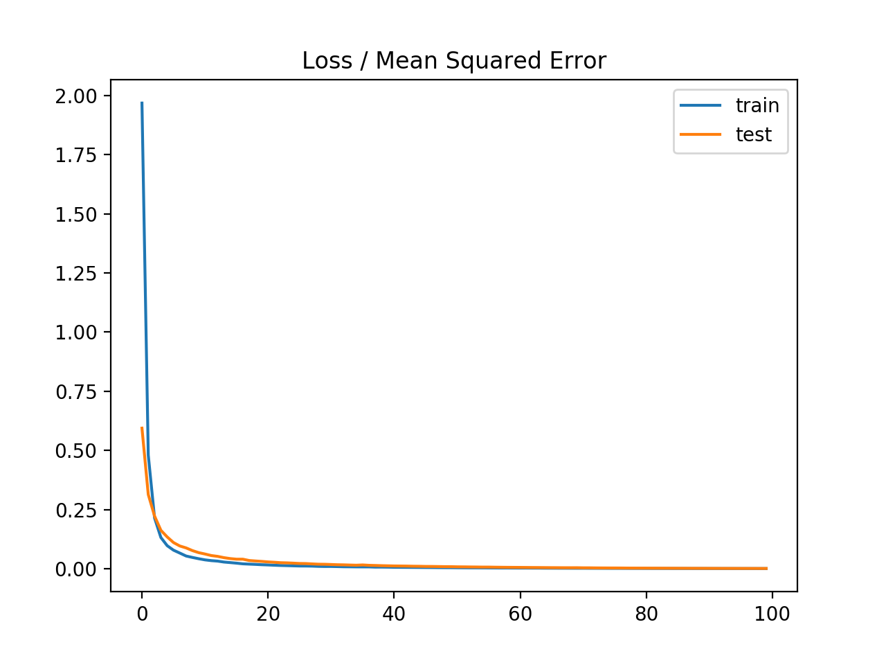
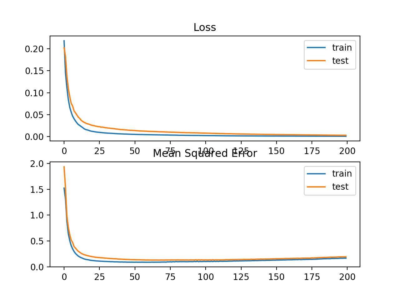
原文地址:How to Choose Loss Functions When Training Deep Learning Neural Networks (Jason Brownlee on January 30, 2019) Updated Oct/2019: Updated for Keras 2.3 and TensorFlow 2.0.Update Jan/2020: Updated for changes in scikit-learn v0.22 API深度学习神经网络采用随机梯度下降优化算法训练。作为优化算法的一部分,模型当前状态的误差必须反复的估计,这需要选择一个误差函数(通常称为损失函数)可以用来估计模型的损失,以便在下次评估时更新权重以减少损失。 神经网络模型从实例中学习从输入到输出的映射,损失函数的选择必须匹配特定预测建模问题(如分类或回归)的框架。此外,输出层的参数选择也必须与所选的损失函数相适应。 在本教程中,您将了解如何为给定的预测问题建模的深度学习神经网络选择一个损失函数。学完本教程后,您将知道: 如何配置回归问题的均方误差和变量的模型;如何配置二元分类的交叉熵和 hinge 损失函数模型;如何配置多类分类的交叉熵和KL散度损失函数模型。在我的新书中,有26个分步教程和完整的源代码,介绍如何用深度学习模型更快地训练、减少过拟合和更好地预测。 教程概述 本教程分为三个部分: 回归的损失函数 均方误差损失/Mean Squared Error Loss平均平方对数误差损失/Mean Squared Logarithmic Error Loss平均绝对误差损失/Mean Absolute Error Loss 二值分类损失函数 二叉熵/Binary Cross-EntropyHinge损失/Hinge LossSquared Hinge损失/Squared Hinge Loss 多类分类损失函数 多类交叉熵损失/Multi-Class Cross-Entropy Loss稀疏多类交叉熵损失/Sparse Multiclass Cross-Entropy LossKullback Leibler散度损失/Kullback Leibler Divergence Loss我们将着重于如何选择和实现不同的损失功能。更多关于损失函数的理论,请看帖子:Loss and Loss Functions for Training Deep Learning Neural Networks 回归损失函数回归预测建模问题预测一个实值量。在本节中,我们将研究适合于回归预测建模问题的损失函数。本次研究,我们将使用scikit-learn库在make_regression()函数中提供的标准回归问题生成器,给定一定数量的输入变量、统计噪声及其他属性,这个函数将从一个简单回归问题中生成实例。sklearn.datasets.make_regression 我们将使用这个函数来定义一个有20个输入特征的问题:其中10个输入特征是有意义的,10个是无关紧要的。总共随机生成1000个示例。伪随机数生成器将被固定,以确保每一运行代码时我们得到相同的1,000 个实例。 from sklearn.datasets import make_regression # generate regression dataset X, y = make_regression(n_samples=1000, n_features=20, noise=0.1, random_state=1)当实值输入和输出变量被缩放到一个可感知的范围时,神经网络通常表现得更好。对于这个问题,每个输入变量和目标变量都具有高斯分布;因此,在这种情况下,标准化数据是可取的,我们可以使用scikit-learn库中的StandardScaler transformer类来实现。在实际的问题中,我们会在训练数据集上准备scaler,并将其应用到训练和测试集上,但为了简单起见,我们会在分割为训练集和测试集之前将所有的数据一起标准化。sklearn.preprocessing.StandardScaler # standardize dataset X = StandardScaler().fit_transform(X) y = StandardScaler().fit_transform(y.reshape(len(y),1))[:,0]标准化后,将数据均匀地分成训练集和测试集, # split into train and test n_train = 500 trainX, testX = X[:n_train, :], X[n_train:, :] trainy, testy = y[:n_train], y[n_train:]我们将定义一个小型多层感知器(MLP)模型来解决这个问题,这为探索不同的损失函数提供基础。 输入层:20个神经元(20个输入特征);隐藏层:25个神经元,激活函数采用rectified linear activation function (ReLU);输出层:一个神经元,激活函数采用线性函数,将会给出一个要预测的实值。 # define model model = Sequential() model.add(Dense(25, input_dim=20, activation='relu', kernel_initializer='he_uniform')) model.add(Dense(1, activation='linear'))Dense就是常用的全连接层,所实现的运算是output = activation(dot(input, kernel)+bias)。其中activation是逐元素计算的激活函数,kernel是本层的权值矩阵,bias为偏置向量,只有当use_bias=True才会添加。Keras官方文档Dense层 模型拟合的学习率为0.01,动量为0.9,均为合理的默认值。训练将执行100个epoch,测试集将在每个epoch结束时进行评估,因此我们可以在运行结束时绘制学习曲线。 opt = SGD(lr=0.01, momentum=0.9) model.compile(loss='...', optimizer=opt) # fit model history = model.fit(trainX, trainy, validation_data=(testX, testy), epochs=100, verbose=0)现在我们已经有了一个问题和模型的基础,我们可以评估适合回归预测建模问题的三个常见损失函数。 虽然在这些例子中使用了MLP,但是在训练CNN和RNN模型进行回归时可以使用相同的损失函数。 Mean Squared Error Loss均方误差(MSE)损失函数是回归问题的默认损失函数。在数学上,如果目标变量的分布是高斯分布,则在最大似然推理框架下,它是优选的损失函数。MSE是首先计算的是损失函数,只有在有充分理由的情况下才会转而计算其他损失函数。 均方误差是预测值和实际值之间的平方差的平均值: M S E = 1 N ∑ i = 1 N ( y i − y ^ i ) 2 MSE=\frac{1}{N}\sum_{i=1}^N(y_i-\hat{y}_i)^2 MSE=N1i=1∑N(yi−y^i)2 无论预测值和实际值的符号是什么,结果总是正的,完美值是0.0。平方意味着大的误差相比小的误差会导致更大的误差,意味着模型会惩罚大的误差。Keras中可以使用均方误差损失函数,在编译模型时指定mse或mean_squared_error作为损失函数。 model.compile(loss='mean_squared_error')建议输出层为目标变量设置一个节点,并使用线性激活函数。 model.add(Dense(1, activation='linear'))下面列出了一个完整的示例,演示关于所描述的回归问题的MLP。 # mlp for regression with mse loss function from sklearn.datasets import make_regression from sklearn.preprocessing import StandardScaler from keras.models import Sequential from keras.layers import Dense from keras.optimizers import SGD from matplotlib import pyplot # generate regression dataset X, y = make_regression(n_samples=1000, n_features=20, noise=0.1, random_state=1) # standardize dataset X = StandardScaler().fit_transform(X) y = StandardScaler().fit_transform(y.reshape(len(y),1))[:,0] # split into train and test n_train = 500 trainX, testX = X[:n_train, :], X[n_train:, :] trainy, testy = y[:n_train], y[n_train:] # define model model = Sequential() model.add(Dense(25, input_dim=20, activation='relu', kernel_initializer='he_uniform')) model.add(Dense(1, activation='linear')) opt = SGD(lr=0.01, momentum=0.9) model.compile(loss='mean_squared_error', optimizer=opt) # fit model history = model.fit(trainX, trainy, validation_data=(testX, testy), epochs=100, verbose=0) # evaluate the model train_mse = model.evaluate(trainX, trainy, verbose=0) test_mse = model.evaluate(testX, testy, verbose=0) print('Train: %.3f, Test: %.3f' % (train_mse, test_mse)) # plot loss during training pyplot.title('Loss / Mean Squared Error') pyplot.plot(history.history['loss'], label='train') pyplot.plot(history.history['val_loss'], label='test') pyplot.legend() pyplot.show()运行这个示例首先打印训练集和测试集上的均方误差。考虑到训练算法的随机性,您的具体结果可能会有所不同。试着运行这个例子几次。在这种情况下,我们可以看到,模型学习的问题实现零误差,至少到小数点后三位。 Train: 0.000, Test: 0.001 还创建了一个线状图,显示了在训练时段内,训练集(蓝色)和测试集(橙色)的均方误差损失。 我们可以看到,模型收敛得相当快,训练和测试性能保持相同。该模型的性能和收敛特性表明,均方误差是一个很好的匹配神经网络学习这个问题。 可能会出现目标值范围很大的回归问题,在预测较大的值时,您可能不希望像均方误差那样严重地惩罚模型。相反,你可以首先计算每个预测值的自然对数,然后计算再其均方误差,这叫做平均平方对数误差损失,简称MSLE。 M S L E = 1 N ∑ i = 1 N ( log ( y ^ i + 1 ) − log ( y i + 1 ) ) 2 MSLE=\frac{1}{N}\sum_{i=1}^N(\log (\hat{y}_i+1)-\log (y_i+1))^2 MSLE=N1i=1∑N(log(y^i+1)−log(yi+1))2 MSLE能够放松对大预测值所带来的大差异的惩罚效应,当模型直接预测未缩放的数据时,它可能是一种更合适的损失度量,我们可以用简单回归问题来演示这个损失函数。可以使用损失函数mean_squared_logmic_error 更新模型,并保持相同的输出层配置。在拟合模型时,我们还将MSE作为评估模型在训练和测试时的性能的指标,并使用它绘制学习曲线。 model.compile(loss='mean_squared_logarithmic_error', optimizer=opt, metrics=['mse'])compile(self, optimizer, loss, metrics=[], loss_weights=None, sample_weight_mode=None)Keras官方文档Model metrics:列表,包含评估模型在训练和测试时的性能的指标,典型用法是metrics=[‘accuracy’]如果要在多输出模型中为不同的输出指定不同的指标,可像该参数传递一个字典,例如metrics={‘ouput_a’: ‘accuracy’} 下面列出了使用MSLE损失函数的完整示例。 # mlp for regression with msle loss function from sklearn.datasets import make_regression from sklearn.preprocessing import StandardScaler from keras.models import Sequential from keras.layers import Dense from keras.optimizers import SGD from matplotlib import pyplot # generate regression dataset X, y = make_regression(n_samples=1000, n_features=20, noise=0.1, random_state=1) # standardize dataset X = StandardScaler().fit_transform(X) y = StandardScaler().fit_transform(y.reshape(len(y),1))[:,0] # split into train and test n_train = 500 trainX, testX = X[:n_train, :], X[n_train:, :] trainy, testy = y[:n_train], y[n_train:] # define model model = Sequential() model.add(Dense(25, input_dim=20, activation='relu', kernel_initializer='he_uniform')) model.add(Dense(1, activation='linear')) opt = SGD(lr=0.01, momentum=0.9) model.compile(loss='mean_squared_logarithmic_error', optimizer=opt, metrics=['mse']) # fit model history = model.fit(trainX, trainy, validation_data=(testX, testy), epochs=100, verbose=0) # evaluate the model _, train_mse = model.evaluate(trainX, trainy, verbose=0) _, test_mse = model.evaluate(testX, testy, verbose=0) print('Train: %.3f, Test: %.3f' % (train_mse, test_mse)) # plot loss during training pyplot.subplot(211) pyplot.title('Loss') pyplot.plot(history.history['loss'], label='train') pyplot.plot(history.history['val_loss'], label='test') pyplot.legend() # plot mse during training pyplot.subplot(212) pyplot.title('Mean Squared Error') pyplot.plot(history.history['mean_squared_error'], label='train') pyplot.plot(history.history['val_mean_squared_error'], label='test') pyplot.legend() pyplot.show()运行这个示例首先打印训练集和测试集上的均方误差。考虑到训练算法的随机性,您的具体结果可能会有所不同,试着多运行这个例子几次。在这种情况下,我们可以看到,该模型导致训练数据集和测试数据集的MSE都略有恶化,这表明该模型可能不能很好的拟合这个问题,因为目标变量的分布是一个标准的高斯分布。 Train: 0.165, Test: 0.184 还创建了一个线状图,显示了在训练时间段内训练集(蓝色)和测试集(橙色)的均方对数误差损失函数,以及一个类似的均方误差图。我们可以看到MSLE在超过100个epoch时算法收敛得很好;MSE可能显示出过度拟合问题的迹象,迅速下降,并从20epoch开始上升。 在一些回归问题上,目标变量的分布可能大多是高斯分布,但也可能有离群值,例如离均值很远(很大或很小)的值。在这种情况下,平均绝对误差损失是一个合适的损失函数,因为它对异常值更有鲁棒性,它是以实际值和预测值之间的绝对差的平均值来计算的。 M A E = 1 N ∑ i = 1 N ∣ y i − y ^ i ∣ MAE=\frac{1}{N}\sum_{i=1}^N|y_i-\hat{y}_i| MAE=N1i=1∑N∣yi−y^i∣ 可以使用损失函数 mean_absolute_error 更新模型,并保持输出层的配置不变。 model.compile(损失=“mean_absolute_error”,优化器选择,指标= [' mse '])下面列出了使用绝对平均误差作为回归测试问题的损失函数的完整例子。 # mlp for regression with mae loss function from sklearn.datasets import make_regression from sklearn.preprocessing import StandardScaler from keras.models import Sequential from keras.layers import Dense from keras.optimizers import SGD from matplotlib import pyplot # generate regression dataset X, y = make_regression(n_samples=1000, n_features=20, noise=0.1, random_state=1) # standardize dataset X = StandardScaler().fit_transform(X) y = StandardScaler().fit_transform(y.reshape(len(y),1))[:,0] # split into train and test n_train = 500 trainX, testX = X[:n_train, :], X[n_train:, :] trainy, testy = y[:n_train], y[n_train:] # define model model = Sequential() model.add(Dense(25, input_dim=20, activation='relu', kernel_initializer='he_uniform')) model.add(Dense(1, activation='linear')) opt = SGD(lr=0.01, momentum=0.9) model.compile(loss='mean_absolute_error', optimizer=opt, metrics=['mse']) # fit model history = model.fit(trainX, trainy, validation_data=(testX, testy), epochs=100, verbose=0) # evaluate the model _, train_mse = model.evaluate(trainX, trainy, verbose=0) _, test_mse = model.evaluate(testX, testy, verbose=0) print('Train: %.3f, Test: %.3f' % (train_mse, test_mse)) # plot loss during training pyplot.subplot(211) pyplot.title('Loss') pyplot.plot(history.history['loss'], label='train') pyplot.plot(history.history['val_loss'], label='test') pyplot.legend() # plot mse during training pyplot.subplot(212) pyplot.title('Mean Squared Error') pyplot.plot(history.history['mean_squared_error'], label='train') pyplot.plot(history.history['val_mean_squared_error'], label='test') pyplot.legend() pyplot.show()运行这个示例首先打印训练集和测试集上的均方误差。考虑到训练算法的随机性,您的具体结果可能会有所不同,试着多运行这个例子几次。在这种情况下,我们可以看到模型学习了这个问题,实现了接近零的误差,至少在小数点后三位。 Train: 0.002, Test: 0.002还创建了一个线状图,显示了在训练时间段内训练集(蓝色)和测试集(橙色)的平均绝对误差损失函数,以及一个类似的均方误差图。在这种情况下,我们可以看到,虽然MSE的动态曲线没有出现很大的影响,MAE也确实收敛,但显示了一个颠簸(bump)的路线。我们知道目标变量是一个没有大异常值的标准高斯分布,所以MAE在这种情况下不是一个很好的拟合。在这个问题上,如果我们不首先缩放目标变量,可能会更合适。 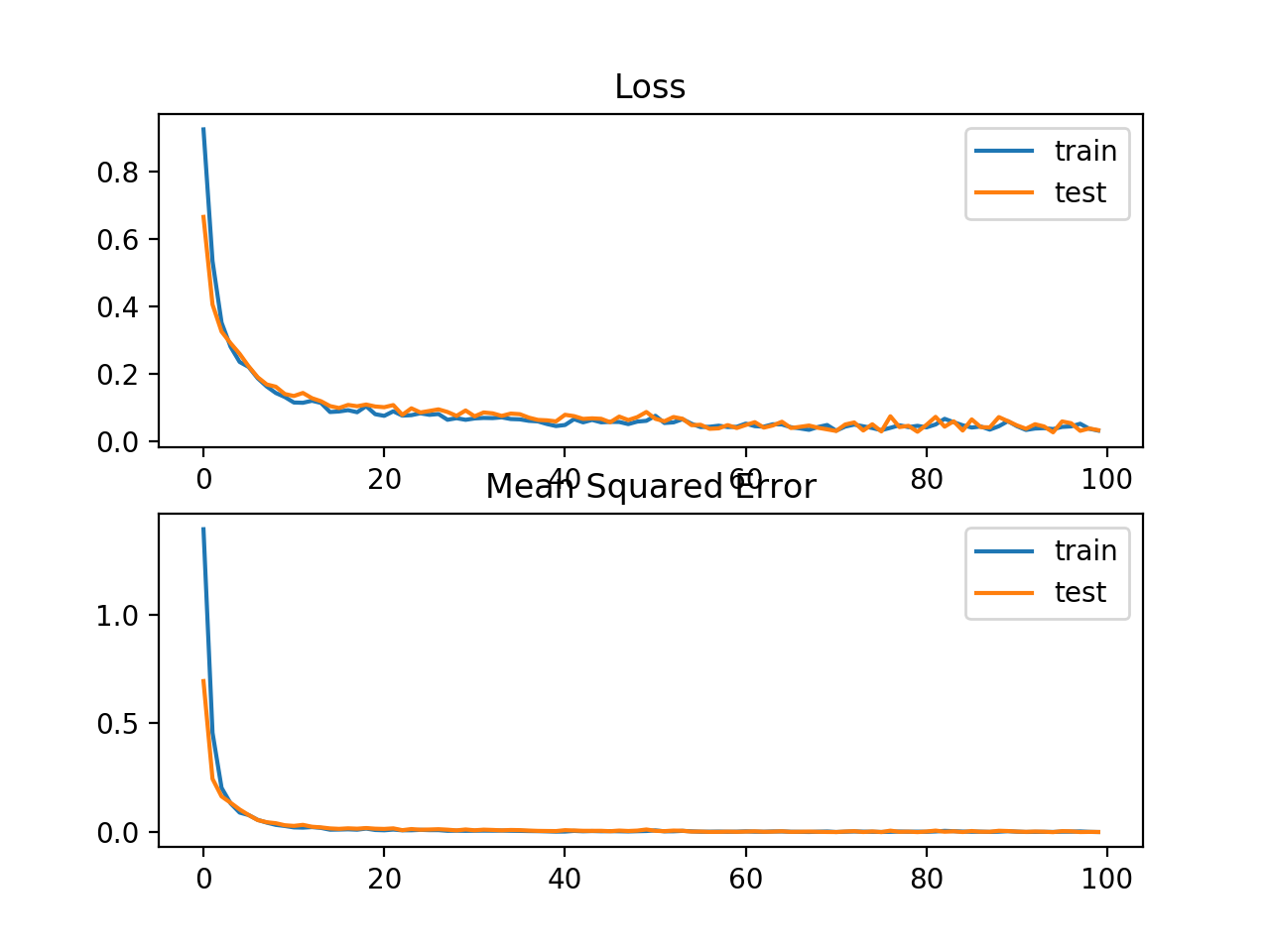 二分类损失函数
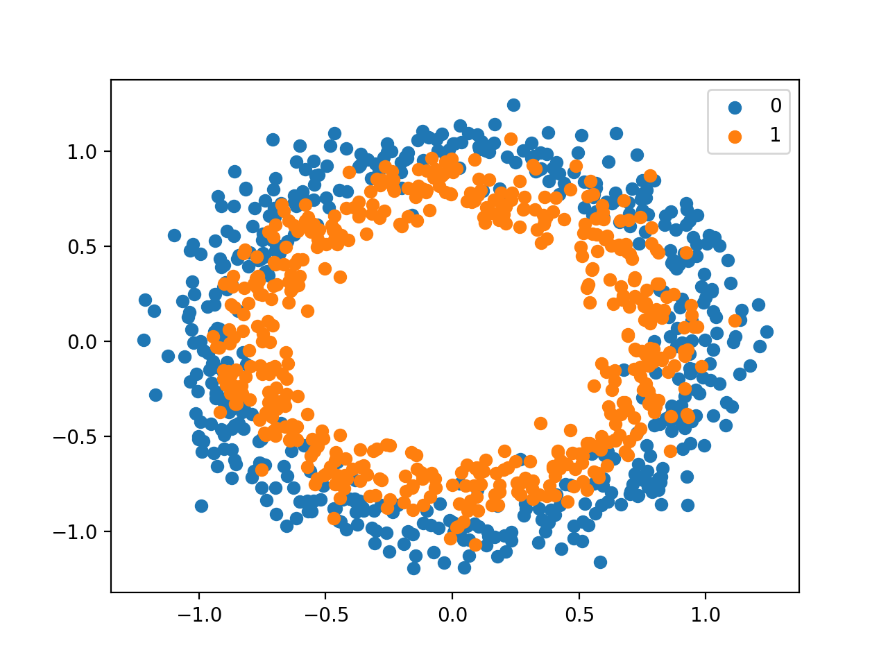
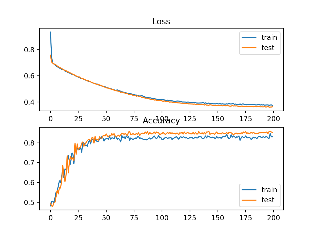
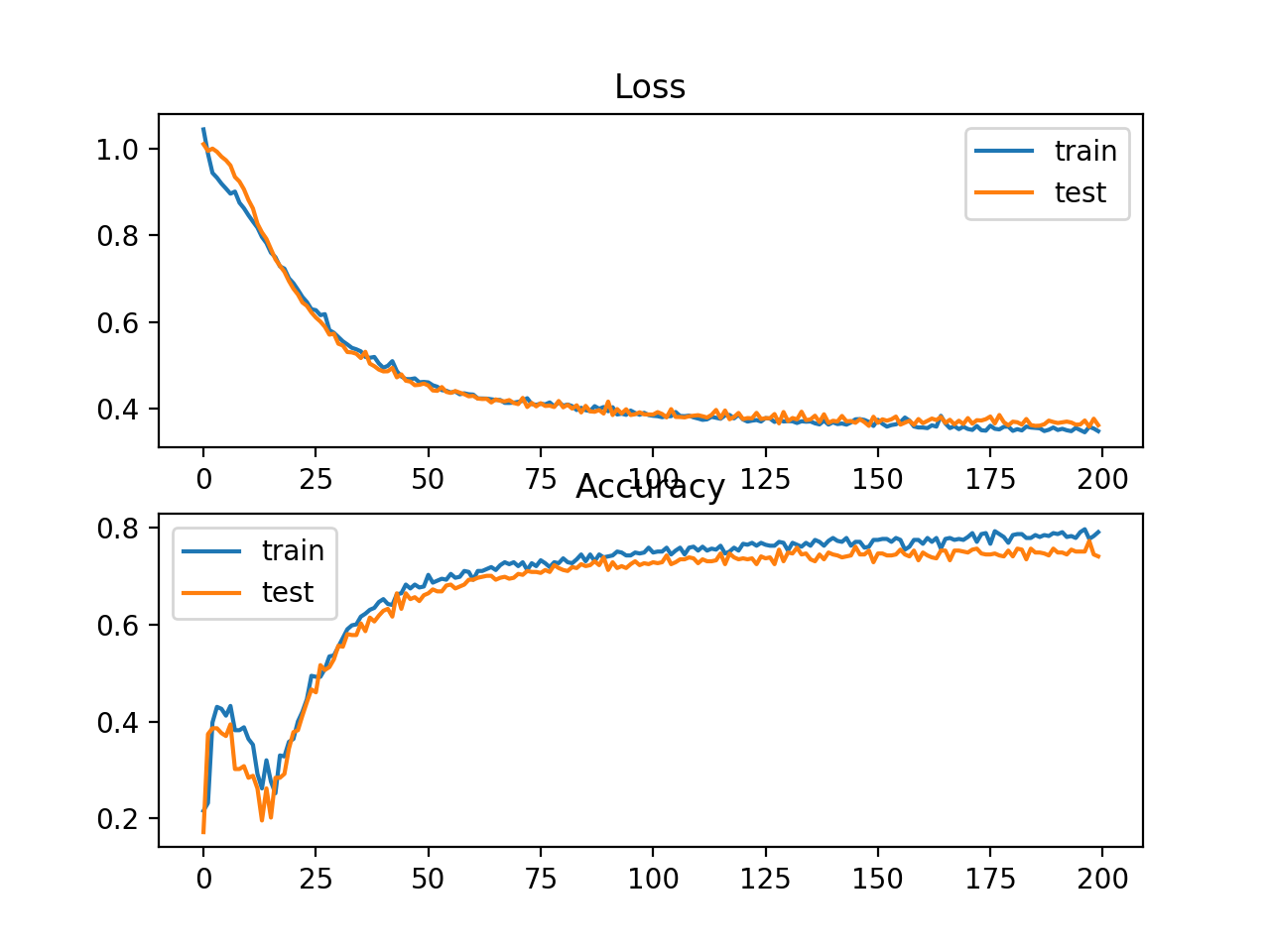
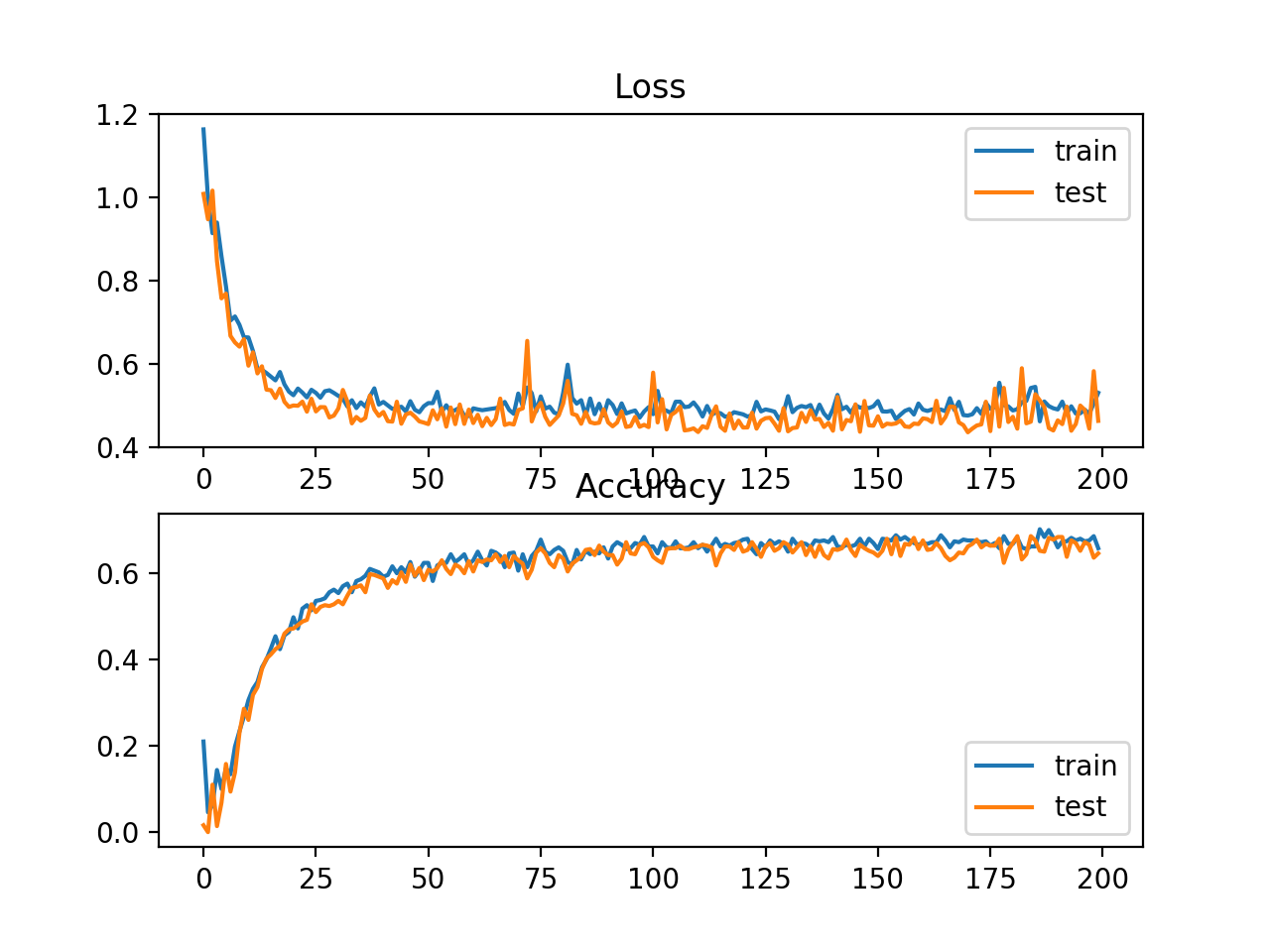
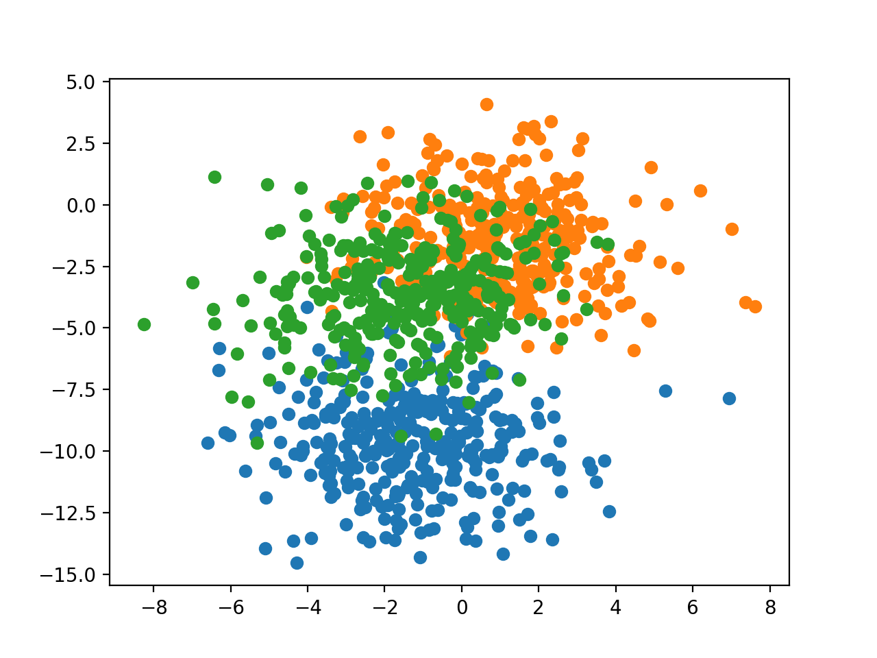
二元分类是指那些例子被指定两个标签之一的预测建模问题,该问题通常定义第一类的值为0、第二类的值1,通过预测实例属于类值1的概率来实现二分类。 在这一节中,我们将研究适和二元分类预测建模问题的损失函数。我们将从scikiti -learn中的圆圈测试问题中生成示例,作为本研究的基础。圆问题涉及从二维平面上的两个同心圆中抽取的样本,其中外圆上的点属于类0,内圆上的点属于类1。统计噪声被添加到样本,以增加模糊度,使问题更具有挑战性的学习。 我们将生成1000个示例并添加10%的统计噪声。伪随机数生成器将被播种相同的值,以确保我们总是得到相同的1,000个示例。 from sklearn.datasets import make_circles # generate circles X, y = make_circles(n_samples=1000, noise=0.1, random_state=1)我们可以创建数据集的散点图来了解我们正在建模的问题。下面列出了完整的示例。 # scatter plot of the circles dataset with points colored by class from sklearn.datasets import make_circles from numpy import where from matplotlib import pyplot # generate circles X, y = make_circles(n_samples=1000, noise=0.1, random_state=1) # select indices of points with each class label for i in range(2): samples_ix = where(y == i) pyplot.scatter(X[samples_ix, 0], X[samples_ix, 1], label=str(i)) pyplot.legend() pyplot.show()运行该示例将创建示例的散点图,其中输入变量定义点的位置,类值定义颜色,类0为蓝色,类1为橙色。 这些点已经合理地在0左右伸缩,几乎在[-1,1]内,我们不会再作标准化。 数据集被均匀地分割成训练集和测试集。 # split into train and test n_train = 500 trainX, testX = X[:n_train, :], X[n_train:, :] trainy, testy = y[:n_train], y[n_train:]可以定义一个简单的MLP模型来解决这个问题:需要对数据集中的两个特性进行输入的包含两个神经元的输入层,一个包含50个神经元的隐藏层,一个经过修正的线性激活函数和一个输出层(需要为损失函数的选择进行配置)。 # define model model = Sequential() model.add(Dense(50, input_dim=2, activation='relu', kernel_initializer='he_uniform')) model.add(Dense(1, activation='...'))模型拟合采用随机梯度下降,合理的默认学习率为0.01,动量为0.9。 opt = SGD(lr=0.01, momentum=0.9) model.compile(loss='...', optimizer=opt, metrics=['accuracy'])我们将对200个训练时期的模型进行拟合,并针对每个时期结束时的损失和准确性评估模型的性能,以便我们可以绘制学习曲线。 # fit model history = model.fit(trainX, trainy, validation_data=(testX, testy), epochs=200, verbose=0)现在我们有了一个问题和模型的基础,我们可以看看评估三个常见的损失函数是适合二分类预测建模问题。 虽然在这些例子中使用了一个MLP,但是在训练CNN和RNN模型进行二值分类时可以使用相同的损失函数。 Binary Cross-Entropy交叉熵是二分类问题的默认的损失函数,它用于目标值在 { 0 , 1 } \{0,1\} {0,1}集合中的二分类。在数学上,它是最大似然推理框架下的优选损失函数。交叉熵损失函数是二分类问题首先计算的损失函数,只有在有充分理由的情况下才会转而计算其他损失函数。 交叉熵将计算一个分数,对实际概率分布和预测概率分布之间的平均差异求和,用于预测第1类。分数最小化,完美的交叉熵值为0。 B C E L o s s = − 1 N ∑ i = 1 N [ y i log P ( y ^ i = 1 ) + ( 1 − y i ) log ( 1 − P ( y ^ i = 1 ) ) ] BCELoss=-\frac{1}{N}\sum_{i=1}^N\left[y_i \log P(\hat{y}_i=1)+(1-y_i)\log (1-P(\hat{y}_i=1))\right] BCELoss=−N1i=1∑N[yilogP(y^i=1)+(1−yi)log(1−P(y^i=1))] 在Keras中,可以通过在编译模型时指定binary_crossentropy来指定交叉熵作为损失函数。 model.compile(loss='binary_crossentropy', optimizer=opt, metrics=['accuracy'])该功能要求输出层配置一个单一节点和一个“sigmoid”激活,以预测类1的概率。 model.add(Dense(1, activation='sigmoid'))下面是一个完整的例子与交叉熵损失的MLP的二圆二分类问题。 # mlp for the circles problem with cross entropy loss from sklearn.datasets import make_circles from keras.models import Sequential from keras.layers import Dense from keras.optimizers import SGD from matplotlib import pyplot # generate 2d classification dataset X, y = make_circles(n_samples=1000, noise=0.1, random_state=1) # split into train and test n_train = 500 trainX, testX = X[:n_train, :], X[n_train:, :] trainy, testy = y[:n_train], y[n_train:] # define model model = Sequential() model.add(Dense(50, input_dim=2, activation='relu', kernel_initializer='he_uniform')) model.add(Dense(1, activation='sigmoid')) opt = SGD(lr=0.01, momentum=0.9) model.compile(loss='binary_crossentropy', optimizer=opt, metrics=['accuracy']) # fit model history = model.fit(trainX, trainy, validation_data=(testX, testy), epochs=200, verbose=0) # evaluate the model _, train_acc = model.evaluate(trainX, trainy, verbose=0) _, test_acc = model.evaluate(testX, testy, verbose=0) print('Train: %.3f, Test: %.3f' % (train_acc, test_acc)) # plot loss during training pyplot.subplot(211) pyplot.title('Loss') pyplot.plot(history.history['loss'], label='train') pyplot.plot(history.history['val_loss'], label='test') pyplot.legend() # plot accuracy during training pyplot.subplot(212) pyplot.title('Accuracy') pyplot.plot(history.history['accuracy'], label='train') pyplot.plot(history.history['val_accuracy'], label='test') pyplot.legend() pyplot.show()运行这个示例首先打印训练集和测试集上的均方误差。考虑到训练算法的随机性,您的具体结果可能会有所不同,试着多运行这个例子几次。在这种情况下,我们可以看到模型对问题的学习相当好,在训练数据集上的准确率约为83%,在测试数据集上的准确率约为85%,得分相当接近,表明模型可能没有过拟合或欠拟合。 Train: 0.836, Test: 0.852 还绘制了两个线图,顶部是训练集(蓝色)和测试集(橙色)在不同时期的交叉熵损失,底部的图显示不同时期的分类精度。从图中可以看出,训练过程收敛得很好。考虑到概率分布之间的误差的连续性质,Loss曲线是平滑的,而accuracy曲线有小的波动,训练集和测试集中给出的例子最终只能被预测为正确或不正确,提供较少粒度的性能反馈。 标签值 y i ∈ { − 1 , 1 } y_i\in\{-1,1\} yi∈{−1,1},预测值 y ^ = w x + b ∈ R \hat{y}=wx+b\in\mathbb{R} y^=wx+b∈R,对于任一样本,定义hinge损失函数为: h i n g e L o s s = max { 0 , 1 − y i ⋅ y ^ i } = max { 0 , 1 − y i ⋅ ( w x i + b ) } hingeLoss=\max\{0,1-y_i\cdot \hat{y}_i\}=\max\{0,1-y_i\cdot (wx_i+b)\} hingeLoss=max{0,1−yi⋅y^i}=max{0,1−yi⋅(wxi+b)} Hinge损失函数可以替代二分类问题中的交叉熵损失函数,主要用于支持向量机(SVM)模型。 Hinge损失函数用于目标值在 { − 1 , 1 } \{- 1,1\} {−1,1}集合中的二分类,它鼓励实例使用正确的符号,当实际的类值和预测的类值之间的符号有差异时,会产生更大的误差。关于Hinge损失函数的性能结果是混合的,有时在二分类问题上的性能优于交叉熵。 首先,必须修改目标变量,使其具有集合 { − 1 , 1 } \{- 1,1\} {−1,1}中的值。 # change y from {0,1} to {-1,1} y[where(y == 0)] = -1使用Hinge损失函数可以在compile函中指定loss为"hinge"。 model.compile(loss='hinge', optimizer=opt, metrics=['accuracy'])最后,网络的输出层必须配置为具有双曲正切激活函数的单个节点,能够输出范围为 [ − 1 , 1 ] [- 1,1] [−1,1]的单个值。 model.add(Dense(1, activation='tanh'))下面是一个完整的例子与Hinge损失函数的MLP为两个圆二分类问题列出。 # mlp for the circles problem with hinge loss from sklearn.datasets import make_circles from keras.models import Sequential from keras.layers import Dense from keras.optimizers import SGD from matplotlib import pyplot from numpy import where # generate 2d classification dataset X, y = make_circles(n_samples=1000, noise=0.1, random_state=1) # change y from {0,1} to {-1,1} y[where(y == 0)] = -1 # split into train and test n_train = 500 trainX, testX = X[:n_train, :], X[n_train:, :] trainy, testy = y[:n_train], y[n_train:] # define model model = Sequential() model.add(Dense(50, input_dim=2, activation='relu', kernel_initializer='he_uniform')) model.add(Dense(1, activation='tanh')) opt = SGD(lr=0.01, momentum=0.9) model.compile(loss='hinge', optimizer=opt, metrics=['accuracy']) # fit model history = model.fit(trainX, trainy, validation_data=(testX, testy), epochs=200, verbose=0) # evaluate the model _, train_acc = model.evaluate(trainX, trainy, verbose=0) _, test_acc = model.evaluate(testX, testy, verbose=0) print('Train: %.3f, Test: %.3f' % (train_acc, test_acc)) # plot loss during training pyplot.subplot(211) pyplot.title('Loss') pyplot.plot(history.history['loss'], label='train') pyplot.plot(history.history['val_loss'], label='test') pyplot.legend() # plot accuracy during training pyplot.subplot(212) pyplot.title('Accuracy') pyplot.plot(history.history['accuracy'], label='train') pyplot.plot(history.history['val_accuracy'], label='test') pyplot.legend() pyplot.show()运行这个示例首先打印训练集和测试集上的均方误差。考虑到训练算法的随机性,您的具体结果可能会有所不同,试着多运行这个例子几次。在这种情况下,我们可以看到比使用交叉熵略差的性能,选择的模型配置在训练集和测试集上的精度低于80%。 Train: 0.792, Test: 0.740 还绘制了两个线图,顶部是训练集(蓝色)和测试集(橙色)在不同时期的Hinge损失,底部的图显示不同时期的分类精度。Hinge损失曲线表明,模型收敛,在两个数据集上都有合理的损失。分类精度的图也显示了收敛的迹象,尽管低于期望的水平。 铰链(Hinge)损失函数有许多扩展,经常是SVM模型的研究主题。一个流行的扩展称为平方铰链损失,即简单计算铰链损失的平方。它具有平滑损失函数表面的效果,从而在数值上更容易处理。如果在给定的二分类问题上使用铰链损失确实会导致更好的性能,那平方铰链损失很可能是合适的。 与使用铰链损失函数一样,目标变量必须修改为取值于集合 { − 1 , 1 } \{- 1,1\} {−1,1}。 # change y from {0,1} to {-1,1} y[where(y == 0)] = -1在定义模型时,可以在compile()函数中指定为squared_hinge来使用平方铰链损失。 model.compile(loss='squared_hinge', optimizer=opt, metrics=['accuracy'])最后,输出层必须使用具有双曲正切激活函数的单个节点,该双曲正切激活函数能够输出 [ − 1 , 1 ] [- 1,1] [−1,1]范围内的连续值。 model.add(Dense(1, activation='tanh'))下面列出了一个完整的例子,一个MLP与平方铰链损失函数的二圆二分类问题。 # mlp for the circles problem with squared hinge loss from sklearn.datasets import make_circles from keras.models import Sequential from keras.layers import Dense from keras.optimizers import SGD from matplotlib import pyplot from numpy import where # generate 2d classification dataset X, y = make_circles(n_samples=1000, noise=0.1, random_state=1) # change y from {0,1} to {-1,1} y[where(y == 0)] = -1 # split into train and test n_train = 500 trainX, testX = X[:n_train, :], X[n_train:, :] trainy, testy = y[:n_train], y[n_train:] # define model model = Sequential() model.add(Dense(50, input_dim=2, activation='relu', kernel_initializer='he_uniform')) model.add(Dense(1, activation='tanh')) opt = SGD(lr=0.01, momentum=0.9) model.compile(loss='squared_hinge', optimizer=opt, metrics=['accuracy']) # fit model history = model.fit(trainX, trainy, validation_data=(testX, testy), epochs=200, verbose=0) # evaluate the model _, train_acc = model.evaluate(trainX, trainy, verbose=0) _, test_acc = model.evaluate(testX, testy, verbose=0) print('Train: %.3f, Test: %.3f' % (train_acc, test_acc)) # plot loss during training pyplot.subplot(211) pyplot.title('Loss') pyplot.plot(history.history['loss'], label='train') pyplot.plot(history.history['val_loss'], label='test') pyplot.legend() # plot accuracy during training pyplot.subplot(212) pyplot.title('Accuracy') pyplot.plot(history.history['accuracy'], label='train') pyplot.plot(history.history['val_accuracy'], label='test') pyplot.legend() pyplot.show()在这种情况下,我们可以看到,对于这个问题和所选择的模型配置,铰链平方损失可能并不合适,导致训练集和测试集上的分类精度低于70%。 Train: 0.682, Test: 0.646 还绘制了两个线图,顶部是训练集(蓝色)和测试集(橙色)在不同时期的铰链损失的平方,底部的图显示不同时期的分类精度。Loss曲线显示,模型确实收敛了,但误差曲面的形状不像其他损失函数那样平滑,在其他损失函数中,权重的微小变化会导致损失的巨大变化。 多类分类是指将实例分配到两个以上类中的一个的预测建模问题。该问题通常被定义为预测一个整数值,其中每个类被分配一个从0到 ( n u m _ c l a s s e s − 1 ) (num\_classes - 1) (num_classes−1)的唯一整数值,该问题通常被实现为预测实例属于每个已知类的概率。 在这一节中,我们将研究损失函数是适合于多类分类预测建模问题。我们将使用blobs问题作为研究的基础。scikit-learn提供的make_blobs()函数提供了一种方法,给定类和输入特征的数量,生成实例。我们将使用这个函数为一个有2个输入变量的3类分类问题生成1000个示例。伪随机数生成器将被一致地种子化,以便在每次运行代码时生成相同的1,000个示例。 # generate dataset X, y = make_blobs(n_samples=1000, centers=3, n_features=2, cluster_std=2, random_state=2)这两个输入变量可以作为二维平面上点的x坐标和y坐标。下面的示例根据它们的类成员关系创建了整个数据集着色点的散点图。 # scatter plot of blobs dataset from sklearn.datasets import make_blobs from numpy import where from matplotlib import pyplot # generate dataset X, y = make_blobs(n_samples=1000, centers=3, n_features=2, cluster_std=2, random_state=2) # select indices of points with each class label for i in range(3): samples_ix = where(y == i) pyplot.scatter(X[samples_ix, 0], X[samples_ix, 1]) pyplot.show()运行该示例将创建一个散点图,显示数据集中的1,000个示例,其中示例分别属于0、1和2个类,颜色分别为蓝色、橙色和绿色。 输入特征服从高斯分布,标准化数据有益于模型性能提高;不过,为了简洁起见,在本例中我们将保持这些值不缩放。 数据集被均匀地分为训练集和测试集。 # split into train and test n_train = 500 trainX, testX = X[:n_train, :], X[n_train:, :] trainy, testy = y[:n_train], y[n_train:]一个小型MLP模型将被用作探索损失函数的基础。该模型期望有两个输入变量,隐藏层有50个节点,并采用修正的线性激活函数(ReLU),输出层必须根据损失函数的选择定制。 # define model model = Sequential() model.add(Dense(50, input_dim=2, activation='relu', kernel_initializer='he_uniform')) model.add(Dense(..., activation='...'))模型采用随机梯度下降法拟合,默认学习率为0.01,动量为0.9。 # compile model opt = SGD(lr=0.01, momentum=0.9) model.compile(loss='...', optimizer=opt, metrics=['accuracy'])模型将在训练集上拟合100个epoch,测试集将被用作验证数据集,允许我们在每个训练epoch结束时评估训练集和测试集上的损失和分类精度,并绘制学习曲线。 # fit model history = model.fit(trainX, trainy, validation_data=(testX, testy), epochs=100, verbose=0)现在我们有了一个问题和模型的基础,我们可以看看评估三个常见的损失函数是适合一个多类分类预测建模问题。虽然在这些例子中使用了一个MLP,但是在训练CNN和RNN模型进行多类分类时可以使用相同的损失函数。 Multi-Class Cross-Entropy Loss交叉熵是多类分类问题的默认损失函数。在这种情况下,它用于多类分类,其中目标值在 { 0 , 1 , 3 , … , n } \{0,1,3,…,n\} {0,1,3,…,n}集合中,其中每个类被分配一个唯一的整数值。在数学上,它是最大似然推理框架下的优选损失函数。交叉熵损失函数是多分类问题首先计算的损失函数,只有在有充分理由的情况下才会改变。 交叉熵将计算一个分数,对问题中所有类的实际概率分布和预测概率分布的平均差值求和。分数最小化,完美的交叉熵值为0。Keras中可以通过在编译模型时指定categorical_crossentropy来使用交叉熵损失函数。 − 1 N ∑ i = 1 N ∑ k = 1 K y i , k log P ( y i ^ = k ) -\frac{1}{N}\sum_{i=1}^N\sum_{k=1}^Ky_{i,k}\log P(\hat{y_i}=k) −N1i=1∑Nk=1∑Kyi,klogP(yi^=k) 其中, y i , k y_{i,k} yi,k为0,1变量,取值为1表示第 i i i个样本属于第 k k k类, K K K为类别个数, N N N为样本个数。 model.compile(loss='categorical_crossentropy', optimizer=opt, metrics=['accuracy'])该函数要求输出层配置n个节点(每个类一个),在本例中是3个节点,以及一个‘softmax’激活,以便预测每个类的概率。 model.add(Dense(3, activation='softmax'))反过来,这意味着目标变量必须是热编码的。这是为了确保每个示例对实际类值的期望概率为1.0,对所有其他类值的期望概率为0.0。这可以使用Keras中的to_categorical() 函数来实现。 # one hot encode output variable y = to_categorical(y)下面列出了多类blob分类问题中具有交叉熵损失的MLP的完整例子。 # mlp for the blobs multi-class classification problem with cross-entropy loss from sklearn.datasets import make_blobs from keras.layers import Dense from keras.models import Sequential from keras.optimizers import SGD from keras.utils import to_categorical from matplotlib import pyplot # generate 2d classification dataset X, y = make_blobs(n_samples=1000, centers=3, n_features=2, cluster_std=2, random_state=2) # one hot encode output variable y = to_categorical(y) # split into train and test n_train = 500 trainX, testX = X[:n_train, :], X[n_train:, :] trainy, testy = y[:n_train], y[n_train:] # define model model = Sequential() model.add(Dense(50, input_dim=2, activation='relu', kernel_initializer='he_uniform')) model.add(Dense(3, activation='softmax')) # compile model opt = SGD(lr=0.01, momentum=0.9) model.compile(loss='categorical_crossentropy', optimizer=opt, metrics=['accuracy']) # fit model history = model.fit(trainX, trainy, validation_data=(testX, testy), epochs=100, verbose=0) # evaluate the model _, train_acc = model.evaluate(trainX, trainy, verbose=0) _, test_acc = model.evaluate(testX, testy, verbose=0) print('Train: %.3f, Test: %.3f' % (train_acc, test_acc)) # plot loss during training pyplot.subplot(211) pyplot.title('Loss') pyplot.plot(history.history['loss'], label='train') pyplot.plot(history.history['val_loss'], label='test') pyplot.legend() # plot accuracy during training pyplot.subplot(212) pyplot.title('Accuracy') pyplot.plot(history.history['accuracy'], label='train') pyplot.plot(history.history['val_accuracy'], label='test') pyplot.legend() pyplot.show()在这种情况下,我们可以看到模型的表现很好,训练数据集的分类准确率约为84%,测试数据集的分类准确率约为82%。 Train: 0.840, Test: 0.822还绘制了两个线图,顶部是训练集(蓝色)和测试集(橙色)在不同时期的交叉熵损失,底部的图显示不同时期的分类精度。在这种情况下,交叉熵和准确率的线图都显示了良好的收敛行为,尽管有点颠簸。如果没有过拟合或过拟合的迹象,模型可以配置得很好。在这种情况下,学习率或批量大小可能会被调优以均匀收敛的平滑性。 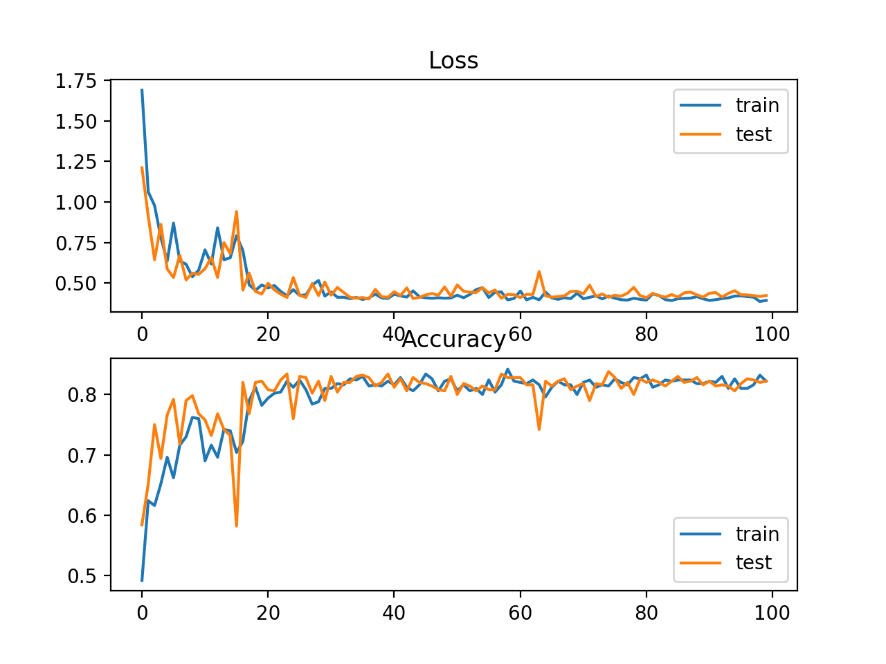 Sparse Multiclass Cross-Entropy Loss
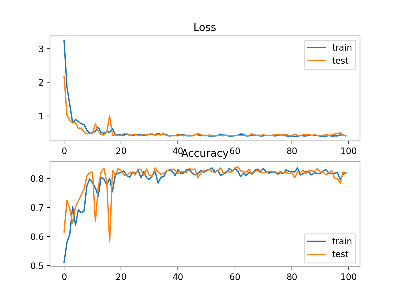
当使用交叉熵处理具有大量标签的分类问题时,一个可能产生问题的原因是独热编码的过程。例如,在词汇表中预测单词可能有数万或数十万个类别,每个标签对应一个类别。这可能意味着,每个训练示例的目标元素可能需要一个热编码向量,其中包含成千上万个零值,这需要大量内存。 稀疏交叉熵解决了这个问题,通过执行相同的交叉熵计算误差,而不要求训练时的目标变量是一个独热编码。在keras中,通过在调用compile()函数时使用sparse_categorical_crossentropy,可以将稀疏交叉熵用于多类分类。 model.compile(loss='sparse_categorical_crossentropy', optimizer=opt, metrics=['accuracy'])该函数要求输出层配置n个节点(每个类一个),在本例中是3个节点,以及一个‘softmax’激活,以便预测每个类的概率。 model.add(Dense(3, activation='softmax'))这种损失函数的一个好处是不需要目标变量的独热编码。 下面是在blobs多类分类问题上训练一个具有稀疏交叉熵的MLP的完整例子。 # mlp for the blobs multi-class classification problem with sparse cross-entropy loss from sklearn.datasets import make_blobs from keras.layers import Dense from keras.models import Sequential from keras.optimizers import SGD from matplotlib import pyplot # generate 2d classification dataset X, y = make_blobs(n_samples=1000, centers=3, n_features=2, cluster_std=2, random_state=2) # split into train and test n_train = 500 trainX, testX = X[:n_train, :], X[n_train:, :] trainy, testy = y[:n_train], y[n_train:] # define model model = Sequential() model.add(Dense(50, input_dim=2, activation='relu', kernel_initializer='he_uniform')) model.add(Dense(3, activation='softmax')) # compile model opt = SGD(lr=0.01, momentum=0.9) model.compile(loss='sparse_categorical_crossentropy', optimizer=opt, metrics=['accuracy']) # fit model history = model.fit(trainX, trainy, validation_data=(testX, testy), epochs=100, verbose=0) # evaluate the model _, train_acc = model.evaluate(trainX, trainy, verbose=0) _, test_acc = model.evaluate(testX, testy, verbose=0) print('Train: %.3f, Test: %.3f' % (train_acc, test_acc)) # plot loss during training pyplot.subplot(211) pyplot.title('Loss') pyplot.plot(history.history['loss'], label='train') pyplot.plot(history.history['val_loss'], label='test') pyplot.legend() # plot accuracy during training pyplot.subplot(212) pyplot.title('Accuracy') pyplot.plot(history.history['accuracy'], label='train') pyplot.plot(history.history['val_accuracy'], label='test') pyplot.legend() pyplot.show()在这种情况下,我们可以看到模型取得了很好的性能。事实上,如果多次重复这个实验,稀疏交叉熵和非稀疏交叉熵的平均性能应该是相当的。 Train: 0.832, Test: 0.818 我们还绘制了两个线图,顶部是训练集(蓝色)和测试集(橙色)在不同时期的稀疏交叉熵损失,底部的图显示不同时期的分类精度。在这种情况下,loss曲线和classification accuracy曲线显示了较好收敛性。 Kullback Leibler散度,或简称KL散度,度量了一个概率分布如何不同于基线分布。KL散度损失为0表明分布是相同的。实际上,KL散度的行为与交叉熵非常相似。它计算如果使用预测的概率分布来近似期望的目标概率分布,会有多少信息丢失(以比特为单位)。 KL散度损失函数更常用于学习模型来近似一个更复杂的函数,而不仅仅是简单的多分类问题,例如在自动编码器的情况下,用于学习密集特征表示下的模型,必须重建原始输入,在这种情况下,首选KL散度损失。然而,它可以用于多分类,这时它在功能上等同于多类交叉熵。 在Keras中,可以通过在compile()函数中指定kullback_leibler_divergence使用KL散度损失。 model.compile(loss='kullback_leibler_divergence', optimizer=opt, metrics=['accuracy'])与交叉熵一样,输出层配置了n个节点(每个类一个),在本例中是3个节点,以及一个“softmax”激活,以便预测每个类的概率。此外,与分类交叉熵一样,我们必须对目标变量进行热编码,使其类值的期望概率为1.0,其他所有类值的期望概率为0.0。 # one hot encode output variable y = to_categorical(y)下面是一个完整的例子,训练一个MLP与KL散度损失的blob多类分类问题。 # mlp for the blobs multi-class classification problem with kl divergence loss from sklearn.datasets import make_blobs from keras.layers import Dense from keras.models import Sequential from keras.optimizers import SGD from keras.utils import to_categorical from matplotlib import pyplot # generate 2d classification dataset X, y = make_blobs(n_samples=1000, centers=3, n_features=2, cluster_std=2, random_state=2) # one hot encode output variable y = to_categorical(y) # split into train and test n_train = 500 trainX, testX = X[:n_train, :], X[n_train:, :] trainy, testy = y[:n_train], y[n_train:] # define model model = Sequential() model.add(Dense(50, input_dim=2, activation='relu', kernel_initializer='he_uniform')) model.add(Dense(3, activation='softmax')) # compile model opt = SGD(lr=0.01, momentum=0.9) model.compile(loss='kullback_leibler_divergence', optimizer=opt, metrics=['accuracy']) # fit model history = model.fit(trainX, trainy, validation_data=(testX, testy), epochs=100, verbose=0) # evaluate the model _, train_acc = model.evaluate(trainX, trainy, verbose=0) _, test_acc = model.evaluate(testX, testy, verbose=0) print('Train: %.3f, Test: %.3f' % (train_acc, test_acc)) # plot loss during training pyplot.subplot(211) pyplot.title('Loss') pyplot.plot(history.history['loss'], label='train') pyplot.plot(history.history['val_loss'], label='test') pyplot.legend() # plot accuracy during training pyplot.subplot(212) pyplot.title('Accuracy') pyplot.plot(history.history['accuracy'], label='train') pyplot.plot(history.history['val_accuracy'], label='test') pyplot.legend() pyplot.show()在这种情况下,我们看到的性能与交叉熵损失的结果类似,在这种情况下,训练集和测试集的准确率约为82%。 Train: 0.822, Test: 0.822还绘制了两个线图,顶部是训练集(蓝色)和测试集(橙色)集在不同时期的KL散度损失,底部的图显示不同时期的分类精度。在这种情况下,图显示了良好的收敛行为的损失和分类精度。考虑到测量的相似性,交叉熵的评估很可能会导致几乎相同的行为。 |

【本文地址】