|
目录
0.学习目标
1.图像分割
2.固定阈值法
3.自动阈值法
3.1自适应阈值法
3.2迭代法阈值分割
3.3Otsu大津法
4.图像边缘提取
4.1图像梯度
4.2模板卷积
4.3梯度图
4.4梯度算子
4.4.1Roberts交叉算子
4.4.2Prewitt算子
4.4.3Sobel算子
4.5Canny边缘检测算法
5.连通区域分析算法
5.1连通区域概要
5.2Two-Pass算法
6.区域生长算法
7.分水岭算法
0.学习目标

1.图像分割

 2.固定阈值法 2.固定阈值法
直方图双峰法

固定阈值分割

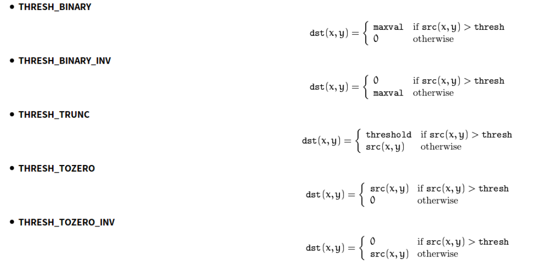
 常用的阈值方法: 常用的阈值方法:
代码:
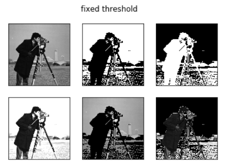
5种不同的阈值方法分割结果对比
#导入第三方包
import cv2
from matplotlib import pyplot as plt
#opencv读取图像
img = cv2.imread('./image/person.png',0)
#5种阈值法图像分割
ret, thresh1 = cv2.threshold(img, 127, 255, cv2.THRESH_BINARY)
ret, thresh2 = cv2.threshold(img, 127, 255, cv2.THRESH_BINARY_INV)
ret, thresh3 = cv2.threshold(img, 127, 255,cv2.THRESH_TRUNC)
ret, thresh4 = cv2.threshold(img, 127, 255, cv2.THRESH_TOZERO)
ret, thresh5 = cv2.threshold(img, 127, 255, cv2.THRESH_TOZERO_INV)
images = [img, thresh1, thresh2, thresh3, thresh4, thresh5]
#使用for循环进行遍历,matplotlib进行显示
for i in range(6):
plt.subplot(2,3, i+1)
plt.imshow(images[i],cmap='gray')
plt.xticks([])
plt.yticks([])
plt.suptitle('fixed threshold')
plt.show()
输出:
3.自动阈值法
3.1自适应阈值法
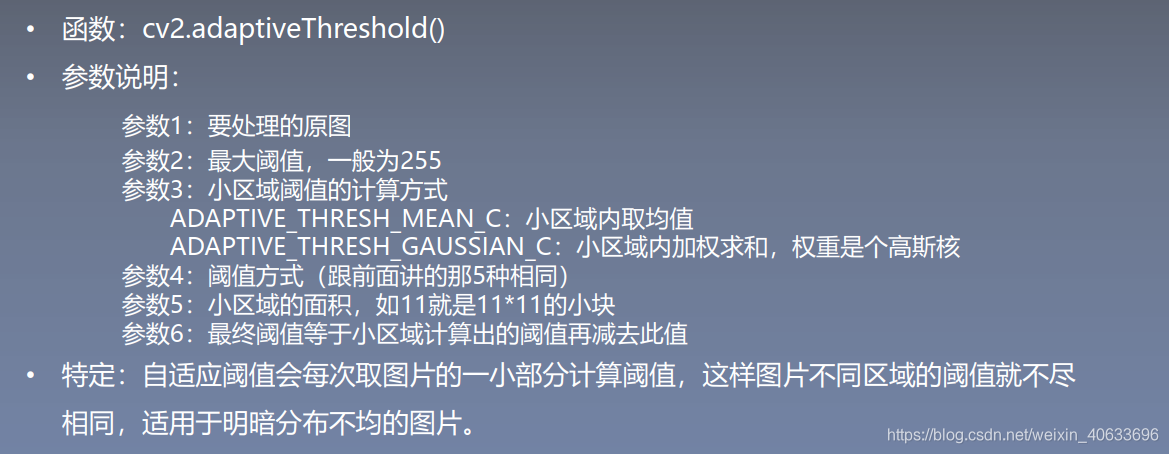 
自适应阈值与固定阈值对比:
#自适应阈值与固定阈值对比
import cv2
import matplotlib.pyplot as plt
img = cv2.imread('./image/paper2.png', 0)
# 固定阈值
ret, th1 = cv2.threshold(img, 127, 255, cv2.THRESH_BINARY)
# 自适应阈值
th2 = cv2.adaptiveThreshold(
img, 255, cv2.ADAPTIVE_THRESH_MEAN_C, cv2.THRESH_BINARY,11, 4)
th3 = cv2.adaptiveThreshold(
img, 255, cv2.ADAPTIVE_THRESH_GAUSSIAN_C, cv2.THRESH_BINARY, 11, 4)
#全局阈值,均值自适应,高斯加权自适应对比
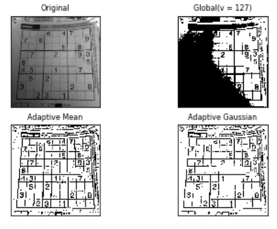
titles = ['Original', 'Global(v = 127)', 'Adaptive Mean', 'Adaptive Gaussian']
images = [img, th1, th2, th3]
for i in range(4):
plt.subplot(2, 2, i + 1), plt.imshow(images[i], 'gray')
plt.title(titles[i], fontsize=8)
plt.xticks([]), plt.yticks([])
plt.show()
输出:
3.2迭代法阈值分割
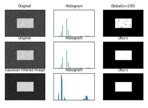
 3.3Otsu大津法 3.3Otsu大津法
   代码: 代码:
import cv2
from matplotlib import pyplot as plt
img = cv2.imread('./image/noisy.png', 0)
# 固定阈值法
ret1, th1 = cv2.threshold(img, 100, 255, cv2.THRESH_BINARY)
# Otsu阈值法
ret2, th2 = cv2.threshold(img, 0, 255, cv2.THRESH_BINARY + cv2.THRESH_OTSU)
# 先进行高斯滤波,再使用Otsu阈值法
blur = cv2.GaussianBlur(img, (5, 5), 0)
ret3, th3 = cv2.threshold(blur, 0, 255, cv2.THRESH_BINARY + cv2.THRESH_OTSU)
images = [img, 0, th1, img, 0, th2, blur, 0, th3]
titles = ['Original', 'Histogram', 'Global(v=100)',
'Original', 'Histogram', "Otsu's",
'Gaussian filtered Image', 'Histogram', "Otsu's"]
for i in range(3):
# 绘制原图
plt.subplot(3, 3, i * 3 + 1)
plt.imshow(images[i * 3], 'gray')
plt.title(titles[i * 3], fontsize=8)
plt.xticks([]), plt.yticks([])
# 绘制直方图plt.hist, ravel函数将数组降成一维
plt.subplot(3, 3, i * 3 + 2)
plt.hist(images[i * 3].ravel(), 256)
plt.title(titles[i * 3 + 1], fontsize=8)
plt.xticks([]), plt.yticks([])
# 绘制阈值图
plt.subplot(3, 3, i * 3 + 3)
plt.imshow(images[i * 3 + 2], 'gray')
plt.title(titles[i * 3 + 2], fontsize=8)
plt.xticks([]), plt.yticks([])
plt.show()
输出:
4.图像边缘提取
4.1图像梯度
梯度

图像梯度
 4.2模板卷积
 4.3梯度图 4.3梯度图
 4.4梯度算子 4.4梯度算子

4.4.1Roberts交叉算子
 4.4.2Prewitt算子 4.4.2Prewitt算子

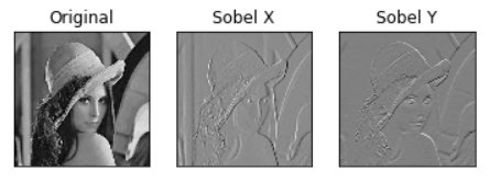
 4.4.3Sobel算子


 代码: 代码:
import numpy as np
import cv2
from matplotlib import pyplot as plt
img = cv2.imread('image/girl2.png',0)
sobelx = cv2.Sobel(img,cv2.CV_64F,1,0,ksize=5)
sobely = cv2.Sobel(img,cv2.CV_64F,0,1,ksize=5)
plt.subplot(1,3,1),plt.imshow(img,cmap = 'gray')
plt.title('Original'), plt.xticks([]), plt.yticks([])
plt.subplot(1,3,2),plt.imshow(sobelx,cmap = 'gray')
plt.title('Sobel X'), plt.xticks([]), plt.yticks([])
plt.subplot(1,3,3),plt.imshow(sobely,cmap = 'gray')
plt.title('Sobel Y'), plt.xticks([]), plt.yticks([])
plt.show()
输出:
4.5Canny边缘检测算法

 代码: 代码:
#加载opencv和numpy
import cv2
import numpy as np
#以灰度图形式读入图像
img = cv2.imread('image/canny.png')
v1 = cv2.Canny(img, 80, 150,(3,3))
v2 = cv2.Canny(img, 50, 100,(5,5))
#np.vstack():在竖直方向上堆叠
#np.hstack():在水平方向上平铺堆叠
ret = np.hstack((v1, v2))
cv2.imshow('img', ret)
cv2.waitKey(0)
cv2.destroyAllWindows()
输出:

5.连通区域分析算法
5.1连通区域概要
 

5.2Two-Pass算法

 6.区域生长算法 6.区域生长算法
区域生长原理
 
7.分水岭算法
分水岭算法概要
 
步骤
 代码: 代码:
# import cv2
"""
完成分水岭算法步骤:
1、加载原始图像
2、阈值分割,将图像分割为黑白两个部分
3、对图像进行开运算,即先腐蚀在膨胀
4、对开运算的结果再进行 膨胀,得到大部分是背景的区域
5、通过距离变换 Distance Transform 获取前景区域
6、背景区域sure_bg 和前景区域sure_fg相减,得到即有前景又有背景的重合区域
7、连通区域处理
8、最后使用分水岭算法
"""
import cv2
import numpy as np
# Step1. 加载图像
img = cv2.imread('image/yezi.jpg')
cv2.imshow("img", img)
cv2.waitKey(0)
cv2.destroyAllWindows()
gray = cv2.cvtColor(img, cv2.COLOR_BGR2GRAY)
# Step2.阈值分割,将图像分为黑白两部分
ret, thresh = cv2.threshold(gray, 0, 255, cv2.THRESH_BINARY_INV + cv2.THRESH_OTSU)
# cv2.imshow("thresh", thresh)
# Step3. 对图像进行“开运算”,先腐蚀再膨胀
kernel = np.ones((3, 3), np.uint8)
opening = cv2.morphologyEx(thresh, cv2.MORPH_OPEN, kernel, iterations=2)
# cv2.imshow("opening", opening)
# Step4. 对“开运算”的结果进行膨胀,得到大部分都是背景的区域
sure_bg = cv2.dilate(opening, kernel, iterations=3)
cv2.imshow("sure_bg", sure_bg)
cv2.waitKey(0)
cv2.destroyAllWindows()
# Step5.通过distanceTransform获取前景区域
dist_transform = cv2.distanceTransform(opening, cv2.DIST_L2, 5) # DIST_L1 DIST_C只能 对应掩膜为3 DIST_L2 可以为3或者5
cv2.imshow("dist_transform", dist_transform)
cv2.waitKey(0)
cv2.destroyAllWindows()
print(dist_transform.max())
ret, sure_fg = cv2.threshold(dist_transform, 0.1 * dist_transform.max(), 255, 0)
# Step6. sure_bg与sure_fg相减,得到既有前景又有背景的重合区域 #此区域和轮廓区域的关系未知
sure_fg = np.uint8(sure_fg)
unknow = cv2.subtract(sure_bg, sure_fg)
cv2.imshow("unknow", unknow)
cv2.waitKey(0)
cv2.destroyAllWindows()
# Step7. 连通区域处理
ret, markers = cv2.connectedComponents(sure_fg,connectivity=8) #对连通区域进行标号 序号为 0 - N-1
#print(markers)
print(ret)
markers = markers + 1 #OpenCV 分水岭算法对物体做的标注必须都 大于1 ,背景为标号 为0 因此对所有markers 加1 变成了 1 - N
#去掉属于背景区域的部分(即让其变为0,成为背景)
# 此语句的Python语法 类似于if ,“unknow==255” 返回的是图像矩阵的真值表。
markers[unknow==255] = 0
# Step8.分水岭算法
markers = cv2.watershed(img, markers) #分水岭算法后,所有轮廓的像素点被标注为 -1
#print(markers)
img[markers == -1] = [0, 0, 255] # 标注为-1 的像素点标 红
cv2.imshow("dst", img)
cv2.waitKey(0)
cv2.destroyAllWindows()
输出:


|