10、图像的几何变换 |
您所在的位置:网站首页 › 图像旋转会引起图像失真吗为什么 › 10、图像的几何变换 |
10、图像的几何变换
|
1.几何变换的基本概念
图像几何变换又称为图像空间变换,它将一副图像中的坐标位置映射到另一幅图像中的新坐标位置。我们学习几何变换就是确定这种空间映射关系,以及映射过程中的变化参数。图像的几何变换改变了像素的空间位置,建立一种原图像像素与变换后图像像素之间的映射关系,通过这种映射关系能够实现下面两种计算: 原图像任意像素计算该像素在变换后图像的坐标位置 变换后图像的任意像素在原图像的坐标位置对于第一种计算,只要给出原图像上的任意像素坐标,都能通过对应的映射关系获得到该像素在变换后图像的坐标位置。将这种输入图像坐标映射到输出的过程称为“向前映射”。反过来,知道任意变换后图像上的像素坐标,计算其在原图像的像素坐标,将输出图像映射到输入的过程称为“向后映射”。但是,在使用向前映射处理几何变换时却有一些不足,通常会产生两个问题:映射不完全,映射重叠 映射不完全 输入图像的像素总数小于输出图像,这样输出图像中的一些像素找不到在原图像中的映射。 上图只有(0,0),(0,2),(2,0),(2,2)四个坐标根据映射关系在原图像中找到了相对应的像素,其余的12个坐标没有有效值。
映射重叠 根据映射关系,输入图像的多个像素映射到输出图像的同一个像素上。 上图只有(0,0),(0,2),(2,0),(2,2)四个坐标根据映射关系在原图像中找到了相对应的像素,其余的12个坐标没有有效值。
映射重叠 根据映射关系,输入图像的多个像素映射到输出图像的同一个像素上。  上图左上角的四个像素(0,0),(0,1),(1,0),(1,1)都会映射到输出图像的(0,0)上,那么(0,0)究竟取那个像素值呢? 上图左上角的四个像素(0,0),(0,1),(1,0),(1,1)都会映射到输出图像的(0,0)上,那么(0,0)究竟取那个像素值呢?
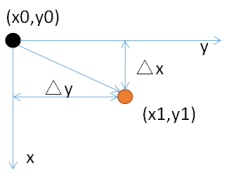
要解决上述两个问题可以使用“向后映射”,使用输出图像的坐标反过来推算改坐标对应于原图像中的坐标位置。这样,输出图像的每个像素都可以通过映射关系在原图像找到唯一对应的像素,而不会出现映射不完全和映射重叠。所以,一般使用向后映射来处理图像的几何变换。从上面也可以看出,向前映射之所以会出现问题,主要是由于图像像素的总数发生了变化,也就是图像的大小改变了。在一些图像大小不会发生变化的变换中,向前映射还是很有效的。 2.图像平移图像的平移变换就是将图像所有的像素坐标分别加上指定的水平偏移量和垂直偏移量。平移变换根据是否改变图像大小分为两种,直接丢弃或者通过加目标图像尺寸的方法使图像能够包含这些点。 2.1平移变换原理假设原来的像素的位置坐标为(x0,y0),经过平移量(△x,△y)后,坐标变为(x1,y1),如下所示: 用数学式子表示可以表示为: x1 = x0 + △x, y1 = y0 + △y; 用矩阵表示为: 本来使用二维矩阵就可以了的,但是为了适应像素、拓展适应性,这里使用三维的向量。 式子中,矩阵: 称为平移变换矩阵(因子),△x和△y为平移量。 2.2 基于OpenCV的实现图像的平移变换实现还是很简单的,这里不再赘述. 平移后图像的大小不变  void GeometricTrans::translateTransform(cv::Mat const& src, cv::Mat& dst, int dx, int dy)
{
CV_Assert(src.depth() == CV_8U);
const int rows = src.rows;
const int cols = src.cols;
dst.create(rows, cols, src.type());
Vec3b *p;
for (int i = 0; i < rows; i++)
{
p = dst.ptr(i);
for (int j = 0; j < cols; j++)
{
//平移后坐标映射到原图像
int x = j - dx;
int y = i - dy;
//保证映射后的坐标在原图像范围内
if (x >= 0 && y >= 0 && x < cols && y < rows)
p[j] = src.ptr(y)[x];
}
}
}
void GeometricTrans::translateTransform(cv::Mat const& src, cv::Mat& dst, int dx, int dy)
{
CV_Assert(src.depth() == CV_8U);
const int rows = src.rows;
const int cols = src.cols;
dst.create(rows, cols, src.type());
Vec3b *p;
for (int i = 0; i < rows; i++)
{
p = dst.ptr(i);
for (int j = 0; j < cols; j++)
{
//平移后坐标映射到原图像
int x = j - dx;
int y = i - dy;
//保证映射后的坐标在原图像范围内
if (x >= 0 && y >= 0 && x < cols && y < rows)
p[j] = src.ptr(y)[x];
}
}
}
平移后图像的大小变化
void GeometricTrans::translateTransformSize(cv::Mat const& src, cv::Mat& dst, int dx, int dy)
{
CV_Assert(src.depth() == CV_8U);
const int rows = src.rows + abs(dy); //输出图像的大小
const int cols = src.cols + abs(dx);
dst.create(rows, cols, src.type());
Vec3b *p;
for (int i = 0; i < rows; i++)
{
p = dst.ptr(i);
for (int j = 0; j < cols; j++)
{
int x = j - dx;
int y = i - dy;
if (x >= 0 && y >= 0 && x < src.cols && y < src.rows)
p[j] = src.ptr(y)[x];
}
}
}
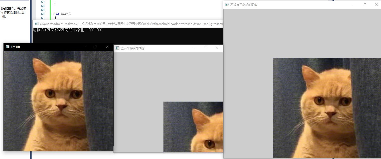
ps:这里图像变换的代码以三通道图像为例,单通道的于此类似,代码中没有做处理。 示例: #include "stdafx.h" #include #include #include #include using namespace std; using namespace cv; void translateTransform(cv::Mat const& src, cv::Mat& dst, int dx, int dy)//平移后大小不变 { CV_Assert(src.depth() == CV_8U); const int rows = src.rows; const int cols = src.cols; dst.create(rows, cols, src.type()); Vec3b *p; for (int i = 0; i < rows; i++) { p = dst.ptr(i); for (int j = 0; j < cols; j++) { //平移后坐标映射到原图像 int x = j - dx; int y = i - dy; //保证映射后的坐标在原图像范围内 if (x >= 0 && y >= 0 && x < cols && y < rows) p[j] = src.ptr(y)[x]; } } } void translateTransformSize(cv::Mat const& src, cv::Mat& dst, int dx, int dy)//平移后大小变化 { CV_Assert(src.depth() == CV_8U); const int rows = src.rows + abs(dy); //输出图像的大小 const int cols = src.cols + abs(dx); dst.create(rows, cols, src.type()); Vec3b *p; for (int i = 0; i < rows; i++) { p = dst.ptr(i); for (int j = 0; j < cols; j++) { int x = j - dx; int y = i - dy; if (x >= 0 && y >= 0 && x < src.cols && y < src.rows) p[j] = src.ptr(y)[x]; } } } int main() { Mat srcImage, dstImage0, dstImage1, dstImage2; int xOffset, yOffset; //x和y方向的平移量 srcImage = imread("111.jpg"); if (!srcImage.data) { cout > yOffset; int rowNumber = srcImage.rows; int colNumber = srcImage.cols; translateTransform(srcImage, dstImage0, xOffset, yOffset); translateTransformSize(srcImage, dstImage1, xOffset, yOffset); imshow("原图像", srcImage); imshow("不丢弃平移后的图像", dstImage0); imshow("丢弃平移后的图像", dstImage1); waitKey(); return 0; }在输入框输入200,200后结果为 3.图像的镜像变换 图像的镜像变换分为两种:水平镜像和垂直镜像。水平镜像以图像垂直中线为轴,将图像的像素进行对换,也就是将图像的左半部和右半部对调。垂直镜像则是以图像的水平中线为轴,将图像的上半部分和下班部分对调。 3.1变换原理 水平变换
2.垂直镜像变换 水平镜像的实现
void GeometricTrans::hMirrorTrans(const Mat &src, Mat &dst)
{
CV_Assert(src.depth() == CV_8U);
dst.create(src.rows, src.cols, src.type());
int rows = src.rows;
int cols = src.cols;
switch (src.channels())
{
case 1:
const uchar *origal;
uchar *p;
for (int i = 0; i < rows; i++){
origal = src.ptr(i);
p = dst.ptr(i);
for (int j = 0; j < cols; j++){
p[j] = origal[cols - 1 - j];
}
}
break;
case 3:
const Vec3b *origal3;
Vec3b *p3;
for (int i = 0; i < rows; i++) {
origal3 = src.ptr(i);
p3 = dst.ptr(i);
for(int j = 0; j < cols; j++){
p3[j] = origal3[cols - 1 - j];
}
}
break;
default:
break;
}
}
分别对三通道图像和单通道图像做了处理,由于比较类似以后的代码只处理三通道图像,不再做特别说明。 在水平镜像变换时,遍历了整个图像,然后根据映射关系对每个像素都做了处理。实际上,水平镜像变换就是将图像坐标的列换到右边,右边的列换到左边,是可以以列为单位做变换的。同样垂直镜像变换也如此,可以以行为单位进行变换。 垂直镜像变换
void GeometricTrans::vMirrorTrans(const Mat &src, Mat &dst)
{
CV_Assert(src.depth() == CV_8U);
dst.create(src.rows, src.cols, src.type());
int rows = src.rows;
for (int i = 0; i < rows; i++)
src.row(rows - i - 1).copyTo(dst.row(i));
}
上面一行代码是变换的核心代码,从原图像中取出第i行,并将其复制到目标图像。 示例: #include "stdafx.h" #include #include #include #include using namespace std; using namespace cv; void hMirrorTrans(const Mat &src, Mat &dst) { CV_Assert(src.depth() == CV_8U); dst.create(src.rows, src.cols, src.type()); int rows = src.rows; int cols = src.cols; switch (src.channels()) { case 1: const uchar *origal; uchar *p; for (int i = 0; i < rows; i++) { origal = src.ptr(i); p = dst.ptr(i); for (int j = 0; j < cols; j++) { p[j] = origal[cols - 1 - j]; } } break; case 3: const Vec3b *origal3; Vec3b *p3; for (int i = 0; i < rows; i++) { origal3 = src.ptr(i); p3 = dst.ptr(i); for (int j = 0; j < cols; j++) { p3[j] = origal3[cols - 1 - j]; } } break; default: break; } } void vMirrorTrans(const Mat &src, Mat &dst) { CV_Assert(src.depth() == CV_8U); dst.create(src.rows, src.cols, src.type()); int rows = src.rows; for (int i = 0; i < rows; i++) src.row(rows - i - 1).copyTo(dst.row(i)); } int main() { Mat srcImage, dstImage, dstImage1;; srcImage = imread("111.jpg"); if (!srcImage.data) { cout = (src.rows - 2)) y1 = src.rows - 2; int y2 = y1 + 1; //根据目标图像的像素点(浮点坐标)找到原始图像中的4个像素点,取距离该像素点最近的一个原始像素值作为该点的值。 assert(0 < x2 && x2 < src.cols && 0 < y2 && y2 < src.rows); std::vector dist(4); dist[0] = distance(x, y, x1, y1); dist[1] = distance(x, y, x2, y1); dist[2] = distance(x, y, x1, y2); dist[3] = distance(x, y, x2, y2); int min_val = dist[0]; int min_index = 0; for (int i = 1; i < dist.size(); ++i) if (min_val > dist[i]) { min_val = dist[i]; min_index = i; } switch (min_index) { case 0: dst.at(i, j) = src.at(y1, x1); break; case 1: dst.at(i, j) = src.at(y1, x2); break; case 2: dst.at(i, j) = src.at(y2, x1); break; case 3: dst.at(i, j) = src.at(y2, x2); break; default: assert(false); } } } double distance(const double x1, const double y1, const double x2, const double y2)//两点之间距离,这里用欧式距离 { return (x1 - x2)*(x1 - x2) + (y1 - y2)*(y1 - y2);//只需比较大小,返回距离平方即可 }最邻近插值只需要对浮点坐标“四舍五入”运算。但是在四舍五入的时候有可能使得到的结果超过原图像的边界(只会比边界大1),所以要进行下修正。 最邻近插值几乎没有多余的运算,速度相当快。但是这种邻近取值的方法是很粗糙的,会造成图像的马赛克、锯齿等现象。 双线性插值 双线性插值的精度要比最邻近插值好很多,相对的其计算量也要大的多。双线性插值的主要思想是计算出浮点坐标像素近似值。那么要如何计算浮点坐标的近似值呢。一个浮点坐标必定会被四个整数坐标所包围,将这个四个整数坐标的像素值按照一定的比例混合就可以求出浮点坐标的像素值。混合比例为距离浮点坐标的距离。 双线性插值使用浮点坐标周围四个像素的值按照一定的比例混合近似得到浮点坐标的像素值。 首先看看线性插值 


下面通过一个例子进行理解: 假设要求坐标为(2.4,3)的像素值P,该点在(2,3)和(3,3)之间,如下图 u和v分别是距离浮点坐标最近两个整数坐标像素在浮点坐标像素所占的比例 P(2.4,3) = u * P(2,3) + v * P(3,3),混合的比例是以距离为依据的,那么u = 0.4,v = 0.6。 接下来看看二维中的双线性插值 
首先在x方向上面线性插值,得到R2、R1 
然后以R2,R1在y方向上面再次线性插值 
同样,通过一个实例进行理解 进行双线性插值运算 这样就可以求得浮点坐标(2.4,3.5)的像素值了。 求浮点坐标像素F,设该浮点坐标周围的4个像素值分别为T1,T2,T3,T4,并且浮点坐标距离其左上角的横坐标的差为m,纵坐标的差为n。 故有 F1 = m * T1 + (1 – m) * T2 F2 = m * T3 + (1 – m) *T4 F = n * F1 + (1 – n) * F2
上面就是双线性插值的基本公式,可以看出,计算每个像素像素值需要进行6次浮点运算。而且,由于浮点坐标有4个坐标近似求得,如果这个四个坐标的像素值差别较大,插值后,会使得图像在颜色分界较为明显的地方变得比较模糊。 OpenCV实现如下: void bilinearIntertpolatioin(cv::Mat& src, cv::Mat& dst, const int rows, const int cols) { //比例尺 const double scale_row = static_cast(src.rows) / rows; const double scale_col = static_cast(src.rows) / cols; //扩展src到dst dst = cv::Mat(rows, cols, src.type()); assert(src.channels() == 1 && dst.channels() == 1); for(int i = 0; i < rows; ++i)//dst的行 for (int j = 0; j < cols; ++j)//dst的列 { //求插值的四个点 double y = (i + 0.5) * scale_row + 0.5; double x = (j + 0.5) * scale_col + 0.5; int x1 = static_cast(x);//col对应x if (x1 >= (src.cols - 2)) x1 = src.cols - 2;//防止越界 int x2 = x1 + 1; int y1 = static_cast(y);//row对应y if (y1 >= (src.rows - 2)) y1 = src.rows - 2; int y2 = y1 + 1; assert(0 < x2 && x2 < src.cols && 0 < y2 && y2 < src.rows); //插值公式,参考维基百科矩阵相乘的公式https://zh.wikipedia.org/wiki/%E5%8F%8C%E7%BA%BF%E6%80%A7%E6%8F%92%E5%80%BC cv::Matx12d matx = { x2 - x, x - x1 }; cv::Matx22d matf = { static_cast(src.at(y1, x1)), static_cast(src.at(y2, x1)), static_cast(src.at(y1, x2)), static_cast(src.at(y2, x2)) }; cv::Matx21d maty = { y2 - y, y - y1 }; auto val = (matx * matf * maty); dst.at(i, j) = val(0,0); } } 3.3示例这里用resize、最近邻域插值和双线性插值(这里给出的两种实现都是基于灰度图的) #include "stdafx.h" #include #include #include double distance(const double x1, const double y1, const double x2, const double y2)//两点之间距离,这里用欧式距离 { return (x1 - x2)*(x1 - x2) + (y1 - y2)*(y1 - y2);//只需比较大小,返回距离平方即可 } void nearestIntertoplation(cv::Mat& src, cv::Mat& dst, const int rows, const int cols) { //比例尺 const double scale_row = static_cast(src.rows) / rows; const double scale_col = static_cast(src.rows) / cols; //扩展src到dst dst = cv::Mat(rows, cols, src.type()); assert(src.channels() == 1 && dst.channels() == 1); for (int i = 0; i < rows; ++i)//dst的行 for (int j = 0; j < cols; ++j)//dst的列 { //求插值的四个点 double y = (i + 0.5) * scale_row + 0.5; double x = (j + 0.5) * scale_col + 0.5; int x1 = static_cast(x);//col对应x if (x1 >= (src.cols - 2)) x1 = src.cols - 2;//防止越界 int x2 = x1 + 1; int y1 = static_cast(y);//row对应y if (y1 >= (src.rows - 2)) y1 = src.rows - 2; int y2 = y1 + 1; //根据目标图像的像素点(浮点坐标)找到原始图像中的4个像素点,取距离该像素点最近的一个原始像素值作为该点的值。 assert(0 < x2 && x2 < src.cols && 0 < y2 && y2 < src.rows); std::vector dist(4); dist[0] = distance(x, y, x1, y1); dist[1] = distance(x, y, x2, y1); dist[2] = distance(x, y, x1, y2); dist[3] = distance(x, y, x2, y2); int min_val = dist[0]; int min_index = 0; for (int i = 1; i < dist.size(); ++i) if (min_val > dist[i]) { min_val = dist[i]; min_index = i; } switch (min_index) { case 0: dst.at(i, j) = src.at(y1, x1); break; case 1: dst.at(i, j) = src.at(y1, x2); break; case 2: dst.at(i, j) = src.at(y2, x1); break; case 3: dst.at(i, j) = src.at(y2, x2); break; default: assert(false); } } } void bilinearIntertpolatioin(cv::Mat& src, cv::Mat& dst, const int rows, const int cols) { //比例尺 const double scale_row = static_cast(src.rows) / rows; const double scale_col = static_cast(src.rows) / cols; //扩展src到dst dst = cv::Mat(rows, cols, src.type()); assert(src.channels() == 1 && dst.channels() == 1); for (int i = 0; i < rows; ++i)//dst的行 for (int j = 0; j < cols; ++j)//dst的列 { //求插值的四个点 double y = (i + 0.5) * scale_row + 0.5; double x = (j + 0.5) * scale_col + 0.5; int x1 = static_cast(x);//col对应x if (x1 >= (src.cols - 2)) x1 = src.cols - 2;//防止越界 int x2 = x1 + 1; int y1 = static_cast(y);//row对应y if (y1 >= (src.rows - 2)) y1 = src.rows - 2; int y2 = y1 + 1; assert(0 < x2 && x2 < src.cols && 0 < y2 && y2 < src.rows); //插值公式,参考维基百科矩阵相乘的公式https://zh.wikipedia.org/wiki/%E5%8F%8C%E7%BA%BF%E6%80%A7%E6%8F%92%E5%80%BC cv::Matx12d matx = { x2 - x, x - x1 }; cv::Matx22d matf = { static_cast(src.at(y1, x1)), static_cast(src.at(y2, x1)), static_cast(src.at(y1, x2)), static_cast(src.at(y2, x2)) }; cv::Matx21d maty = { y2 - y, y - y1 }; auto val = (matx * matf * maty); dst.at(i, j) = val(0, 0); } } int main() { cv::Mat img = cv::imread("111.jpg", 0); if (img.empty()) return -1; cv::Mat dst,dst1,dst2; nearestIntertoplation(img, dst, 600, 600); bilinearIntertpolatioin(img, dst1, 600, 600); resize(img, dst2, dst1.size()); cv::imshow("img", img); cv::imshow("最邻近插值法", dst); cv::imshow("双线性插值", dst1); cv::imshow("resize插值", dst2); cv::waitKey(0); return 0; return 0; }//main
4.图像旋转 4.1旋转原理 图像的旋转就是让图像按照某一点旋转指定的角度。图像旋转后不会变形,但是其垂直对称抽和水平对称轴都会发生改变,旋转后图像的坐标和原图像坐标之间的关系已不能通过简单的加减乘法得到,而需要通过一系列的复杂运算。而且图像在旋转后其宽度和高度都会发生变化,其坐标原点会发生变化。 图像所用的坐标系不是常用的笛卡尔,其左上角是其坐标原点,X轴沿着水平方向向右,Y轴沿着竖直方向向下。而在旋转的过程一般使用旋转中心为坐标原点的笛卡尔坐标系,所以图像旋转的第一步就是坐标系的变换。设旋转中心为(x0,y0),(x’,y’)是旋转后的坐标,(x,y)是旋转后的坐标,则坐标变换如下:
矩阵表示为:
在最终的实现中,常用到的是有缩放后的图像通过映射关系找到其坐标在原图像中的相应位置,这就需要上述映射的逆变换
坐标系变换到以旋转中心为原点后,接下来就要对图像的坐标进行变换。
上图所示,将坐标(x0,y0)顺时针方向旋转a,得到(x1,y1)。 旋转前有:
旋转a后有:
矩阵的表示形式:
其逆变换:
由于在旋转的时候是以旋转中心为坐标原点的,旋转结束后还需要将坐标原点移到图像左上角,也就是还要进行一次变换。这里需要注意的是,旋转中心的坐标(x0,y0)实在以原图像的左上角为坐标原点的坐标系中得到,而在旋转后由于图像的宽和高发生了变化,也就导致了旋转后图像的坐标原点和旋转前的发生了变换。
上边两图,可以清晰的看到,旋转前后图像的左上角,也就是坐标原点发生了变换。 在求图像旋转后左上角的坐标前,先来看看旋转后图像的宽和高。从上图可以看出,旋转后图像的宽和高与原图像的四个角旋转后的位置有关。 设top为旋转后最高点的纵坐标,down为旋转后最低点的纵坐标,left为旋转后最左边点的横坐标,right为旋转后最右边点的横坐标。 旋转后的宽和高为newWidth,newHeight,则可得到下面的关系:
也就很容易的得出旋转后图像左上角坐标(left,top)(以旋转中心为原点的坐标系) 故在旋转完成后要将坐标系转换为以图像的左上角为坐标原点,可由下面变换关系得到:
矩阵表示:
其逆变换:
综合以上,也就是说原图像的像素坐标要经过三次的坐标变换: 将坐标原点由图像的左上角变换到旋转中心 以旋转中心为原点,图像旋转角度a 旋转结束后,将坐标原点变换到旋转后图像的左上角可以得到下面的旋转公式:(x’,y’)旋转后的坐标,(x,y)原坐标,(x0,y0)旋转中心,a旋转的角度(顺时针)
这种由输入图像通过映射得到输出图像的坐标,是向前映射。常用的向后映射是其逆运算
4.2基于OpenCV的实现 得到了上述的旋转公式,实现起来就不是很困难了. Mat nearestNeighRotate(cv::Mat img, float angle) { int len = (int)(sqrtf(pow(img.rows, 2) + pow(img.cols, 2)) + 0.5); Mat retMat = Mat::zeros(len, len, CV_8UC3); float anglePI = angle * CV_PI / 180; int xSm, ySm; for (int i = 0; i < retMat.rows; i++) for (int j = 0; j < retMat.cols; j++) { xSm = (int)((i - retMat.rows / 2)*cos(anglePI) - (j - retMat.cols / 2)*sin(anglePI) + 0.5); ySm = (int)((i - retMat.rows / 2)*sin(anglePI) + (j - retMat.cols / 2)*cos(anglePI) + 0.5); xSm += img.rows / 2; ySm += img.cols / 2; if (xSm >= img.rows || ySm >= img.cols || xSm = img.cols || xSm |


 向前映射 其逆变换为
  向后映射
向后映射 其逆变换为
其逆变换为 

 (2.4,3)的像素值 F1 = m * T1 + (1 – m) * T2 (2.4,4)的像素值 F2 = m * T3 + (1 – m ) * T4 (2.4,3.5)的像素值 F = n * F1 + (1 – n) * F2


【本文地址】
今日新闻 |
推荐新闻 |