|
文章目录
前言一、数据采集与处理1、数据来源2、数据预处理
二、可视化分析(统计学)1.特征分解2.整体关系图(pairplot)3.相关性分析(heatmap)4.参看各因素与count的关系
三、基于机器学习的模型预测1.特征工程2.随机森林算法3.xgboost模型预测
四、GUI界面设计总结
前言
本项目分析了影响单车租赁数的众多因素:年月日期时间、温度、湿度、季节、天气、风速,并对华盛顿地区的单车租赁需求进行预测。 本项目使用的模块:numpy、pandas、matplotlib、seaborn、datatime
一、数据采集与处理
1、数据来源
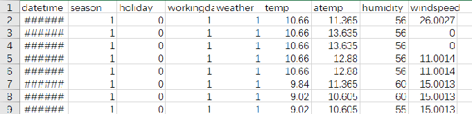
数据平台:Kaggle,一个数据建模和数据分析竞赛平台。 数据链接:https://www.kaggle.com/c/bike-sharing-demand 数据内容:美国华盛顿共享单车租赁数据,数据提供了跨越两年的每天不同时刻单车租赁数据,包含天气信息和日期信息,训练集(train.csv)由每月前19天的数据组成,测试集(test.csv)是每月第20天到当月底的数据。
data_train = pd.read_csv('train.csv')
data_test = pd.read_csv('test.csv')
2、数据预处理
(1)缺失值检查
#缺失值检查
data_train.info()
print('-'*40)
data_test.info()
运行结果: 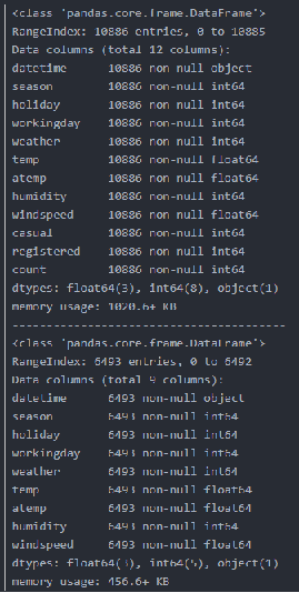 表明数据集没有内容缺失 (2)异常值处理 第一,绘制直方图,观察数据分布情况 表明数据集没有内容缺失 (2)异常值处理 第一,绘制直方图,观察数据分布情况
# 查看是否符合高斯分布
fig,axes = plt.subplots(1,3)
# 设置图形的尺寸,单位为英寸。1英寸等于2.54cm
fig.set_size_inches(18,5)
sns.distplot(data_train['count'],bins=100,ax=axes[0])
sns.distplot(data_train['casual'],bins=100,ax=axes[1])
sns.distplot(data_train['registered'],bins=100,ax=axes[2])

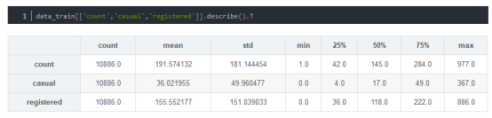
第二,数据统计信息描述
 第三、箱线图(sns.boxplot函数)观察数据分布情况 第三、箱线图(sns.boxplot函数)观察数据分布情况
fig,axes = plt.subplots(1,3)
fig.set_size_inches(12,6)
sns.boxplot(data = data_train['count'],ax=axes[0])
axes[0].set(xlabel='count')
sns.boxplot(data = data_train['casual'], ax=axes[1])
axes[1].set(xlabel='casual')
sns.boxplot(data = data_train['registered'], ax=axes[2])
axes[2].set(xlabel='registered')
 第四,删除异常值(长尾,大值),并做对数log处理 第四,删除异常值(长尾,大值),并做对数log处理
# 去除异常值 将大于μ+3σ的数据值作为异常值
def drop_outlier(data,col):
mask = np.abs(data[col]-data[col].mean())temp(温度)>atemp(体感温度)>humidity(湿度)>month(月份)>season(季节)>year(年份)>weather(天气等级)>windspeed(风速)>workingday(工作日)>weekday(星期几)>day(天数)>(holiday)节假日
4.参看各因素与count的关系
(1)hour
# hour总体变化趋势
date = data_train.groupby(['hour'], as_index=False).agg({'count':'mean',
'registered':'mean',
'casual':'mean'})
fig = plt.figure(figsize=(18,6))
ax = fig.add_subplot(1,1,1)
# 使用总量
plt.plot(date['hour'], date['count'], linewidth=1.3)
# 会员使用量
plt.plot(date['hour'], date['registered'], linewidth=1.3)
# 非会员使用量
plt.plot(date['hour'], date['casual'], linewidth=1.3)
plt.legend()

# 工作日与非工作日下,hour与count的关系
date = data_train.groupby(['workingday','hour'], as_index=False).agg({'count':'mean',
'registered':'mean',
'casual':'mean'})
mask = date['workingday'] == 1
workingday_date= date[mask].drop(['workingday','hour'],axis=1).reset_index(drop=True)
nworkingday_date = date[~mask].drop(['workingday','hour'],axis=1).reset_index(drop=True)
fig, axes = plt.subplots(1,2,sharey = True)
workingday_date.plot(figsize=(15,5),title ='working day',ax=axes[0])
axes[0].set(xlabel='hour')
nworkingday_date.plot(figsize=(15,5),title ='nonworkdays',ax=axes[1])
axes[1].set(xlabel='hour')
 可以看出: *工作日 会员用户(registered)上下班时间是两个用车高峰,而中午也会有一个小高峰,猜测可能是外出午餐的人。 临时用户(casual)起伏比较平缓,高峰期在17点左右。 会员用户(registered)的用车数量远超临时用户(casual)。 *非工作日 租赁数量(count)随时间呈现一个正态分布,高峰在12点左右,低谷在4点左右,且分布比较均匀。 可以看出: *工作日 会员用户(registered)上下班时间是两个用车高峰,而中午也会有一个小高峰,猜测可能是外出午餐的人。 临时用户(casual)起伏比较平缓,高峰期在17点左右。 会员用户(registered)的用车数量远超临时用户(casual)。 *非工作日 租赁数量(count)随时间呈现一个正态分布,高峰在12点左右,低谷在4点左右,且分布比较均匀。
(2)temp
# 按温度取平均值
temp = data_train.groupby(['temp'], as_index=True).agg({'count':'mean',
'registered':'mean',
'casual':'mean'})
temp.plot(figsize=(10,5),title='温度与count的变化趋势')
 (3)humidity (3)humidity
# 湿度
humidity = data_train.groupby(['humidity'], as_index=True).agg({'count':'mean',
'registered':'mean',
'casual':'mean'})
humidity.plot(figsize=(10,5),title='湿度与count的变化趋势')
 (4)month (4)month
# 月使用量变化趋势
date = data_train.groupby(['month'], as_index=False).agg({'count':'mean',
'registered':'mean',
'casual':'mean'})
fig = plt.figure(figsize=(18,6))
ax = fig.add_subplot(1,1,1)
plt.plot(date['month'], date['count'] , linewidth=1.3 , label = '使用总量' )
plt.plot(date['month'], date['registered'] , linewidth=1.3 , label = '会员使用量' )
plt.plot(date['month'], date['casual'] , linewidth=1.3 , label = '非会员使用量' )
plt.legend()
 (5)season (5)season
day_df=data_train.groupby('date').agg({'year':'mean','season':'mean',
'casual':'sum', 'registered':'sum'
,'count':'sum','temp':'mean',
'atemp':'mean'})
season_df = day_df.groupby(['year','season'], as_index=True).agg({'casual':'mean',
'registered':'mean',
'count':'mean'})
temp_df = day_df.groupby(['year','season'], as_index=True).agg({'temp':'mean',
'atemp':'mean'})
fig = plt.figure(figsize=(10,10))
xlables = season_df.index.map(lambda x:str(x))
ax1 = fig.add_subplot(2,1,1)
ax1.set_title('这两年count随季节的总体趋势')
plt.plot(xlables,season_df)
plt.legend(['casual','registered','count'])
ax2 = fig.add_subplot(2,1,2)
ax2.set_title('这两年count随季节的总体趋势')
plt.plot(xlables,temp_df)
plt.legend(['temp','atemp'])

无论是临时用户还是会员用户用车的数量都在秋季迎来高峰,而春季度用户数量最低
(6)weather
weather_df = data_train.groupby('weather',as_index=True).agg({'casual':'mean',
'registered':'mean'})
weather_df.plot.bar(stacked=True)

(7)windspeed
# 风速
# 化为整数型数据
data_train['windspeed'] = data_train['windspeed'].astype(int)
windspeed = data_train.groupby(['windspeed'], as_index=True).agg({'count':'mean',
'registered':'mean',
'casual':'mean'})
windspeed.plot(figsize=(10,8))
 (8)日期(直方图) (8)日期(直方图)  
三、基于机器学习的模型预测
1.特征工程
首先,数据异常值处理,并取对数
train = pd.read_csv('train.csv')
test = pd.read_csv('test.csv')
#训练集去除3倍方差以外数据
train_std = train[np.abs(train['count']-train['count'].mean()) |