|
@创建于:20210324 @修改于:20210324
文章目录
特别说明参考来源包版本号
1、简介2、一次指数平滑2.1 理论介绍2.2 代码展示2.3 参数介绍
3、 二次指数平滑3.1 理论介绍3.1.1 Holt’s linear trend method3.1.2 Damped trend methods
3.2 代码展示3.3 参数介绍
4、 三次指数平滑4.1 理论介绍4.1.1 Holt-Winters’ additive method4.1.2 Holt-Winters’ multiplicative method4.1.3 Holt-Winters’ damped method
4.2 代码展示4.3 参数介绍
5、参数优化和模型选择理论——AIC BIC6、 与 ARIMA 的关系
特别说明
参考来源
本文理论内容转自下面三个博客,它们为同一位作者。代码部分我做了改动。
指数平滑方法简介 个人博客 指数平滑方法简介 简书指数平滑方法简介 CSDN
包版本号
本文测试所用的版本号:
python 3.8.5statsmodels 0.12.2pandas 1.2.2
1、简介
指数平滑(Exponential smoothing)是除了 ARIMA 之外的另一种被广泛使用的时间序列预测方法。 指数平滑即指数移动平均(exponential moving average),是以指数式递减加权的移动平均。各数值的权重随时间指数式递减,越近期的数据权重越高。常用的指数平滑方法有一次指数平滑、二次指数平滑和三次指数平滑。
2、一次指数平滑
2.1 理论介绍
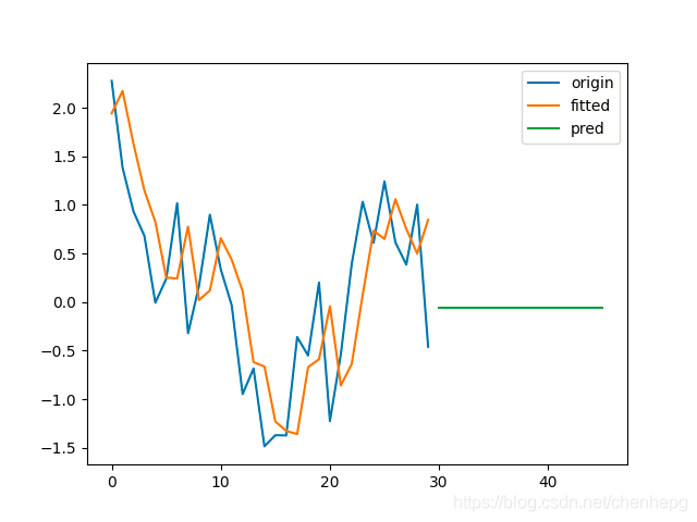
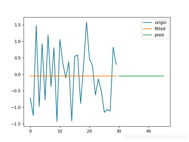
一次指数平滑又叫简单指数平滑(simple exponential smoothing, SES),适合用来预测没有明显趋势和季节性的时间序列。其预测结果是一条水平的直线。模型形如: 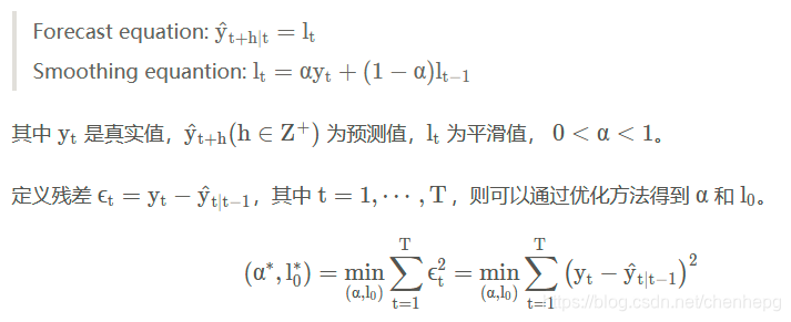
2.2 代码展示
使用 python 的 statsmodels 可以方便地应用该模型:
import numpy as np
import pandas as pd
import matplotlib.pyplot as plt
def ses():
from statsmodels.tsa.holtwinters import SimpleExpSmoothing
number = 30
x1 = np.round(np.linspace(0, 1, number), 4)
y1 = pd.Series(np.multiply(x1, (x1 - 0.5)) + np.random.randn(number))
# fitted部分是直线或者是曲线,受到原始数据影响。
# 多次测试显示,直线的概率高。
# ets1 = SimpleExpSmoothing(endog=y1, initialization_method='estimated')
ets1 = SimpleExpSmoothing(endog=y1, initialization_method='heuristic')
r1 = ets1.fit()
pred1 = r1.predict(start=len(y1), end=len(y1) + len(y1)//2)
pd.DataFrame({
'origin': y1,
'fitted': r1.fittedvalues,
'pred': pred1
}).plot()
plt.savefig('ses.png')
ses()
2.3 参数介绍
Simple Exponential Smoothing
Parameters
----------
endog : array_like
The time series to model.
initialization_method : str, optional
Method for initialize the recursions. One of:
* None
* 'estimated'
* 'heuristic'
* 'legacy-heuristic'
* 'known'
None defaults to the pre-0.12 behavior where initial values
are passed as part of ``fit``. If any of the other values are
passed, then the initial values must also be set when constructing
the model. If 'known' initialization is used, then `initial_level`
must be passed, as well as `initial_trend` and `initial_seasonal` if
applicable. Default is 'estimated'. "legacy-heuristic" uses the same
values that were used in statsmodels 0.11 and earlier.
initial_level : float, optional
The initial level component. Required if estimation method is "known".
If set using either "estimated" or "heuristic" this value is used.
This allows one or more of the initial values to be set while
deferring to the heuristic for others or estimating the unset
parameters.
Fit the model
Parameters
----------
smoothing_level : float, optional
The smoothing_level value of the simple exponential smoothing, if
the value is set then this value will be used as the value.
optimized : bool, optional
Estimate model parameters by maximizing the log-likelihood.
start_params : ndarray, optional
Starting values to used when optimizing the fit. If not provided,
starting values are determined using a combination of grid search
and reasonable values based on the initial values of the data.
initial_level : float, optional
Value to use when initializing the fitted level.
use_brute : bool, optional
Search for good starting values using a brute force (grid)
optimizer. If False, a naive set of starting values is used.
use_boxcox : {True, False, 'log', float}, optional
Should the Box-Cox transform be applied to the data first? If 'log'
then apply the log. If float then use the value as lambda.
remove_bias : bool, optional
Remove bias from forecast values and fitted values by enforcing
that the average residual is equal to zero.
method : str, default "L-BFGS-B"
The minimizer used. Valid options are "L-BFGS-B" (default), "TNC",
"SLSQP", "Powell", "trust-constr", "basinhopping" (also "bh") and
"least_squares" (also "ls"). basinhopping tries multiple starting
values in an attempt to find a global minimizer in non-convex
problems, and so is slower than the others.
minimize_kwargs : dict[str, Any]
A dictionary of keyword arguments passed to SciPy's minimize
function if method is one of "L-BFGS-B" (default), "TNC",
"SLSQP", "Powell", or "trust-constr", or SciPy's basinhopping
or least_squares. The valid keywords are optimizer specific.
Consult SciPy's documentation for the full set of options.
Returns
-------
HoltWintersResults
See statsmodels.tsa.holtwinters.HoltWintersResults.
3、 二次指数平滑
3.1 理论介绍
3.1.1 Holt’s linear trend method
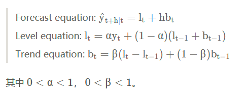
Holt 扩展了简单指数平滑,使其可以用来预测带有趋势的时间序列。直观地看,就是对平滑值的一阶差分(可以理解为斜率)也作一次平滑。模型的预测结果是一条斜率不为0的直线。模型形如:
3.1.2 Damped trend methods
Holt’s linear trend method 得到的预测结果是一条直线,即认为未来的趋势是固定的。对于短期有趋势、长期趋于稳定的序列,可以引入一个阻尼系数 0 |