WGCNA分析教程五

您所在的位置：网站首页 › wgcna分析需要的数据 › WGCNA分析教程五

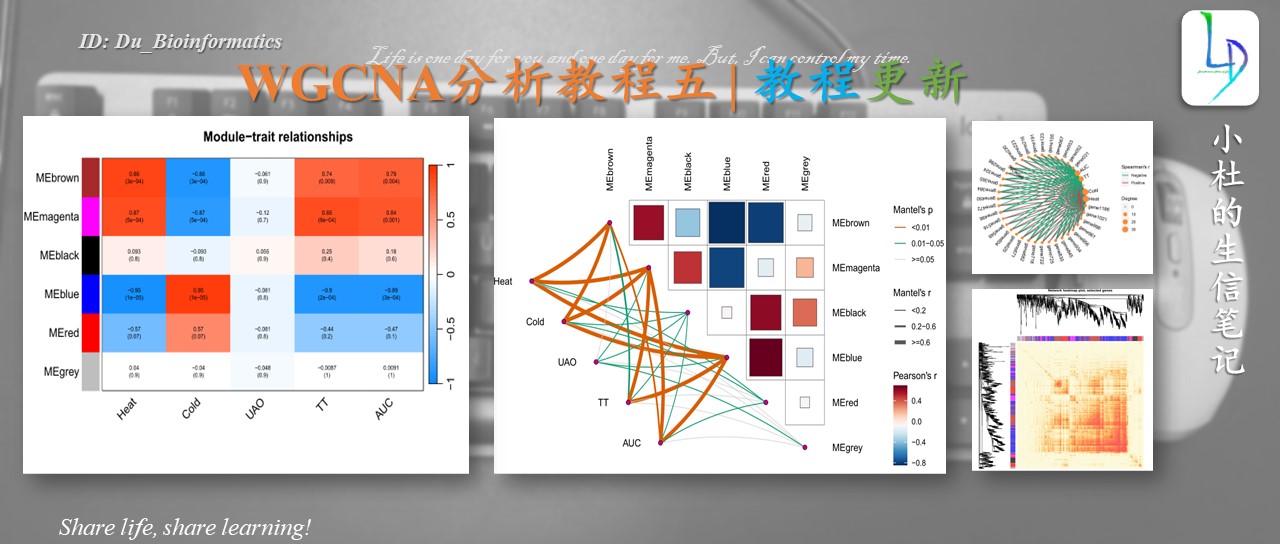
WGCNA分析教程五

2023-11-07 18:24| 来源: 网络整理| 查看: 265

一边学习，一边总结，一边分享！

往期WGCNA分析教程

WGCNA分析 | 全流程分析代码 | 代码一

WGCNA分析 | 全流程分析代码 | 代码二

WGCNA分析 | 全流程分析代码 | 代码四

关于WGCNA分析教程日常更新

学习无处不在，我们的教程会在原有的基础上不断进行更新和添加新的内容，以及不断完善的分析代码。尽最大的能力，让大家拿到代码后直接上手分析。而不需要调整那些看不懂的参数而烦恼（但这仅限于自己的能力范围之内）。

本次WGCNA教程更新，是基于WGCNA分析 | 全流程分析代码 | 代码一的教程。针对原有教程一，增加模块基因文件输出、各模块Hub基因之间的link文件输出(此文件可以直接输入Cytoscape软件，绘制hub基因直接网络图)、相关性共表网络图和共表达基因与性状的相关性网络图

本教程所有图形

![外链图片转存失败,源站可能有防盗链机制,建议将图片保存下来直接上传](https://img-home.csdnimg.cn/images/20230724024159.png?origin_url=https%3A%2F%2Ffiles.mdnice.com%2Fuser%2F40177%2Fa82cb84a-1fe8-4f75-82d9-75be9a8165a4.png%2C!%5B%5D(https%3A%2F%2Fimg-blog.csdnimg.cn%2Fimg_convert%2Fd150713efd9e3dd01d0aea3f79a93c83.png&pos_id=img-rucft6iq-1697730354296)

分析代码

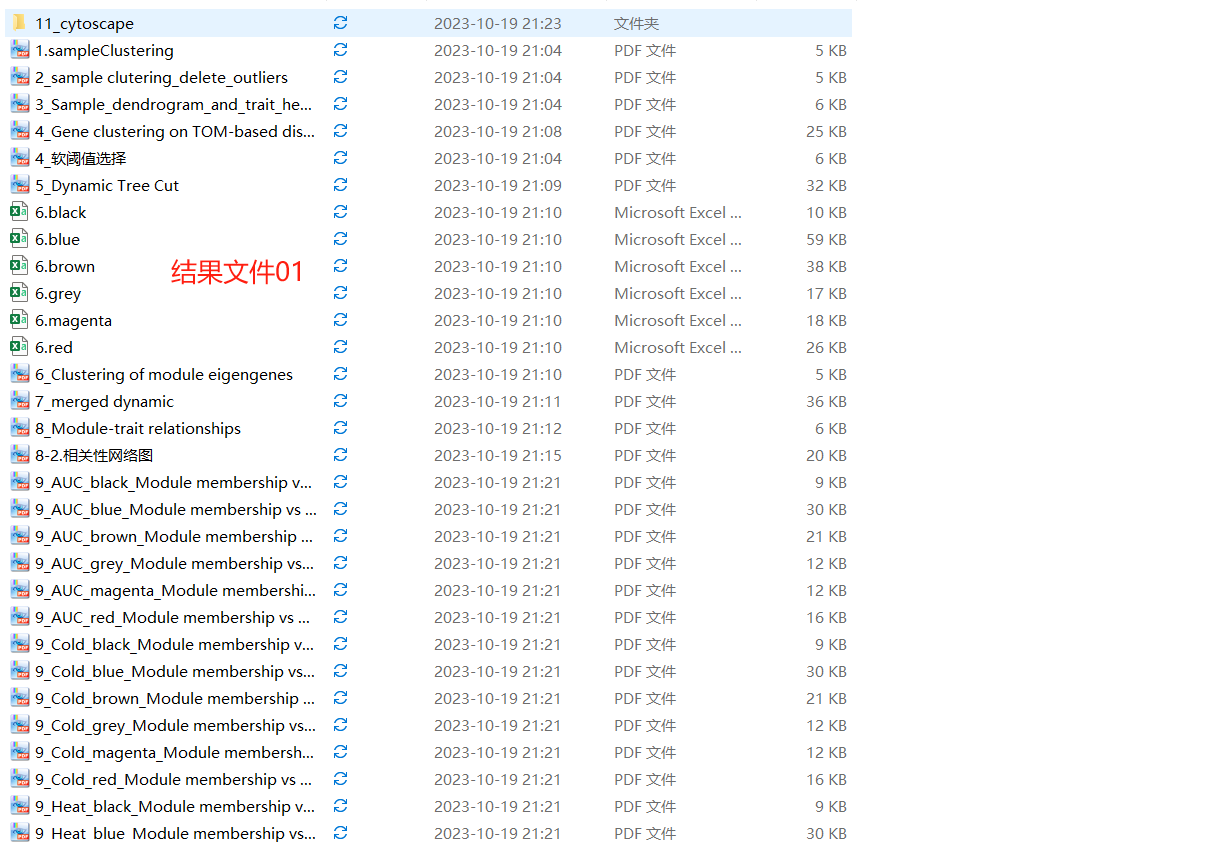
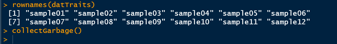
关于WGCNA分析，如果你的数据量较大，建议使用服务期直接分析，本地分析可能导致R崩掉。

设置文件位置 setwd("setwd("E:\\小杜的生信筆記\\2023\\20230217_WGCNA\\WGCNA_05")")

加载分析所需的安装包

install.packages("WGCNA") #BiocManager::install('WGCNA') library(WGCNA) options(stringsAsFactors = FALSE)

注意，如果你想打开多线程分析，可以使用一下代码

enableWGCNAThreads() 一、导入基因表达量数据 ##'@标准化【optional】 ##'@对于数据标准化，根据自己的需求即可，非必要 # WGCNA.fpkm 0) printFlush(paste("Removing genes:", paste(names(datExpr0)[!gsg$goodGenes], collapse = ", "))) if (sum(!gsg$goodSamples)>0) printFlush(paste("Removing samples:", paste(rownames(datExpr0)[!gsg$goodSamples], collapse = ", "))) # Remove the offending genes and samples from the data: datExpr0 = datExpr0[gsg$goodSamples, gsg$goodGenes] }

过滤低于设定的值的基因

##filter meanFPKM=0.5 ###--过滤标准，可以修改 n=nrow(datExpr0) datExpr0[n+1,]=apply(datExpr0[c(1:nrow(datExpr0)),],2,mean) datExpr0=datExpr0[1:n,datExpr0[n+1,] > meanFPKM] # for meanFpkm in row n+1 and it must be above what you set--select meanFpkm>opt$meanFpkm(by rp) filtered_fpkm=t(datExpr0) filtered_fpkm=data.frame(rownames(filtered_fpkm),filtered_fpkm) names(filtered_fpkm)[1]="sample" head(filtered_fpkm) write.table(filtered_fpkm, file="mRNA.filter.txt", row.names=F, col.names=T,quote=FALSE,sep="\t") Sample cluster sampleTree = hclust(dist(datExpr0), method = "average") pdf(file = "1.sampleClustering.pdf", width = 15, height = 8) par(cex = 0.6) par(mar = c(0,6,6,0)) plot(sampleTree, main = "Sample clustering to detect outliers", sub="", xlab="", cex.lab = 2, cex.axis = 1.5, cex.main = 2) ### Plot a line to show the cut #abline(h = 180, col = "red")##剪切高度不确定，故无红线 dev.off() 不过滤数据

如果你的数据不进行过滤直接进行一下操作,此步与前面的操作相同，任选异种即可。

##'@此步这里我们不过滤，直接使用 ## Determine cluster under the line clust = cutreeStatic(sampleTree, cutHeight = 50000, minSize = 10) table(clust) # clust 1 contains the samples we want to keep. keepSamples = (clust!=0) datExpr0 = datExpr0[keepSamples, ] write.table(filtered_fpkm, file="WGCNA.过滤后数据.txt",, row.names=F, col.names=T,quote=FALSE,sep="\t") ### #############Sample cluster########### sampleTree = hclust(dist(datExpr0), method = "average") pdf(file = "1.sampleClustering.pdf", width = 6, height = 4) par(cex = 0.6) par(mar = c(0,6,6,0)) plot(sampleTree, main = "Sample clustering to detect outliers", sub="", xlab="", cex.lab = 2, cex.axis = 1.5, cex.main = 2) ### Plot a line to show the cut #abline(h = 180, col = "red")##剪切高度不确定，故无红线 dev.off() 去除离群值 pdf("2_sample clutering_delete_outliers.pdf", width = 6, height = ) par(cex = 0.6) par(mar = c(0,6,6,0)) cutHeight = 15 ### cut高度 plot(sampleTree, main = "Sample clustering to detect outliers", sub="", xlab="", cex.lab = 2, cex.axis = 1.5, cex.main = 2) + abline(h = cutHeight, col = "red") ###'@"h = 1500"参数为你需要过滤的参数高度 dev.off() 过滤离散样本[optional]

此步可选步骤。

##'@过滤离散样本 ##'@"cutHeight"为过滤参数，与上述图保持一致 clust = cutreeStatic(sampleTree, cutHeight = cutHeight, minSize = 10) keepSamples = (clust==1) datExpr = datExpr0[keepSamples, ] nGenes = ncol(datExpr) nSamples = nrow(datExpr) dim(datExpr) head(datExpr) datExpr[1:11,1:12] 二、导入性状数据 ##'@导入csv格式 traitData = read.csv("TraitData.csv",row.names=1) # ##'@导入txt格式 # traitData = read.table("TraitData.txt",row.names=1,header=T,comment.char = "",check.names=F) head(traitData) allTraits = traitData dim(allTraits) names(allTraits) # 形成一个类似于表达数据的数据框架 fpkmSamples = rownames(datExpr) traitSamples =rownames(allTraits) traitRows = match(fpkmSamples, traitSamples) datTraits = allTraits[traitRows,] rownames(datTraits)

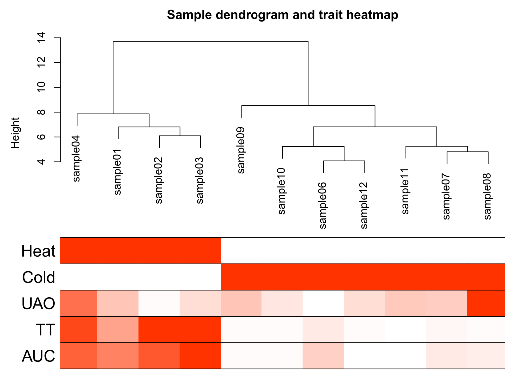
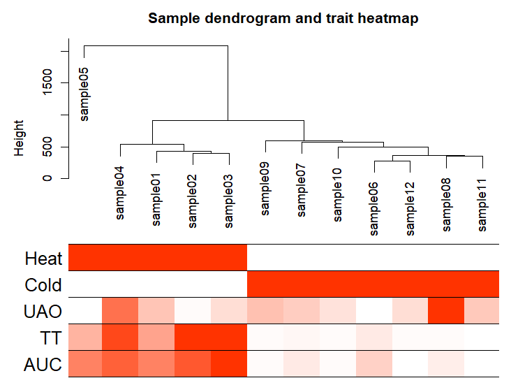
再次样本聚类 sampleTree2 = hclust(dist(datExpr0), method = "average") # Convert traits to a color representation: white means low, red means high, grey means missing entry traitColors = numbers2colors(datTraits, signed = FALSE)

输出样本聚类图

pdf(file="3_Sample_dendrogram_and_trait_heatmap.pdf",width=8 ,height= 6) plotDendroAndColors(sampleTree2, traitColors, groupLabels = names(datTraits), main = "Sample dendrogram and trait heatmap",cex.colorLabels = 1.5, cex.dendroLabels = 1, cex.rowText = 2) dev.off()

三、WGCNA分析（后面都是重点）筛选软阈值 enableWGCNAThreads() # 设置soft-thresholding powers的数量 powers = c(1:30) sft = pickSoftThreshold(datExpr0, powerVector = powers, verbose = 5)

此步骤是比较耗费时间的，静静等待即可。

绘制soft Threshold plot #'@绘制soft power plot pdf(file="4_软阈值选择.pdf",width=12, height = 8) par(mfrow = c(1,2)) cex1 = 0.85 # Scale-free topology fit index as a function of the soft-thresholding power plot(sft$fitIndices[,1], -sign(sft$fitIndices[,3])*sft$fitIndices[,2], xlab="Soft Threshold (power)",ylab="Scale Free Topology Model Fit,signed R^2",type="n", main = paste("Scale independence")); text(sft$fitIndices[,1], -sign(sft$fitIndices[,3])*sft$fitIndices[,2], labels=powers,cex=cex1,col="red"); # this line corresponds to using an R^2 cut-off of h abline(h=0.85,col="red") # Mean connectivity as a function of the soft-thresholding power plot(sft$fitIndices[,1], sft$fitIndices[,5], xlab="Soft Threshold (power)",ylab="Mean Connectivity", type="n", main = paste("Mean connectivity")) text(sft$fitIndices[,1], sft$fitIndices[,5], labels=powers, cex=cex1,col="red") dev.off()

选择softpower

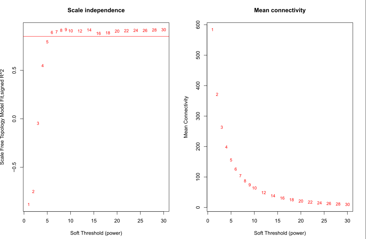
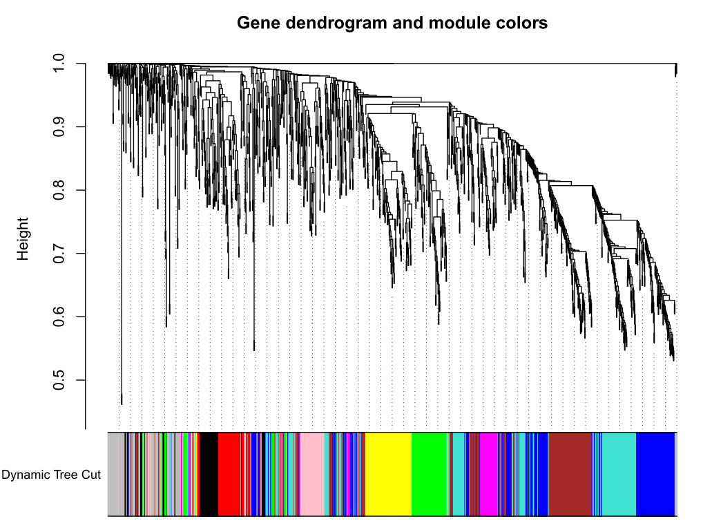
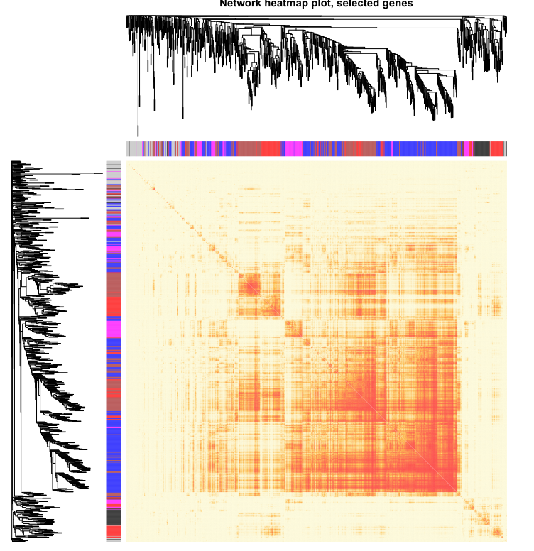
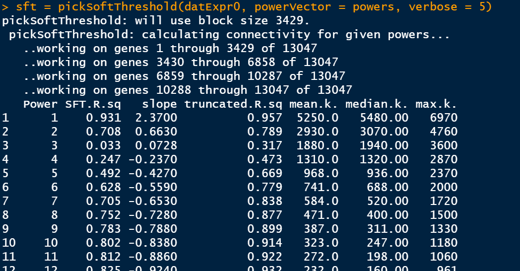
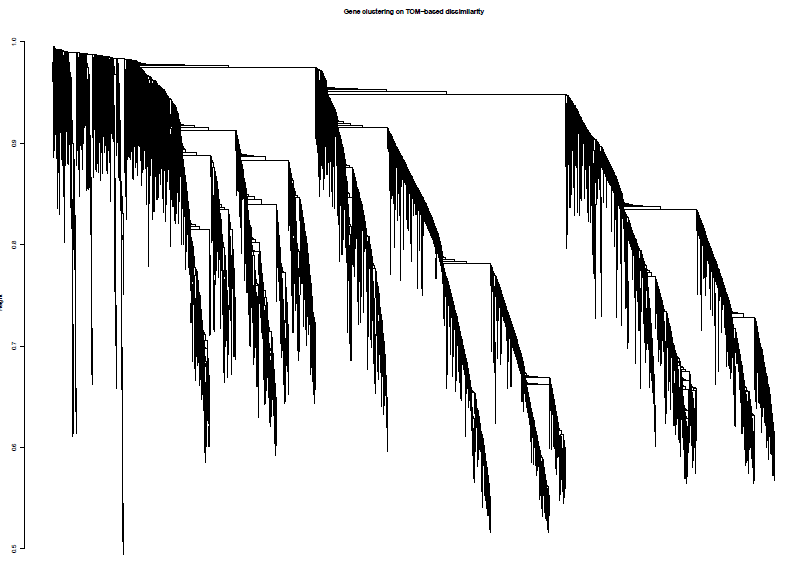
选择softpower是一个玄学的过程，可以直接使用软件自己认为是最好的softpower值，但是不一定你要获得最好结果；其次，我们自己选择自己认为比较好的softpower值，但是，需要自己不断的筛选。因此，从这里开始WGCNA的分析结果就开始受到不同的影响。

## 选择软件认为是最好的softpower值 #softPower =sft$powerEstimate --- # 自己设定softpower值 softPower = 9

继续分析

adjacency = adjacency(datExpr, power = softPower) 将邻接转化为拓扑重叠

这一步建议去服务器上跑，后面的步骤就在服务器上跑吧，数据量太大；如果你的数据量较小，本地也就可以

TOM = TOMsimilarity(adjacency); dissTOM = 1-TOM geneTree = hclust(as.dist(dissTOM), method = "average"); 绘制聚类树(树状图) pdf(file="4_Gene clustering on TOM-based dissimilarity.pdf",width=6,height=4) plot(geneTree, xlab="", sub="", main = "Gene clustering on TOM-based dissimilarity", labels = FALSE, hang = 0.04) dev.off()

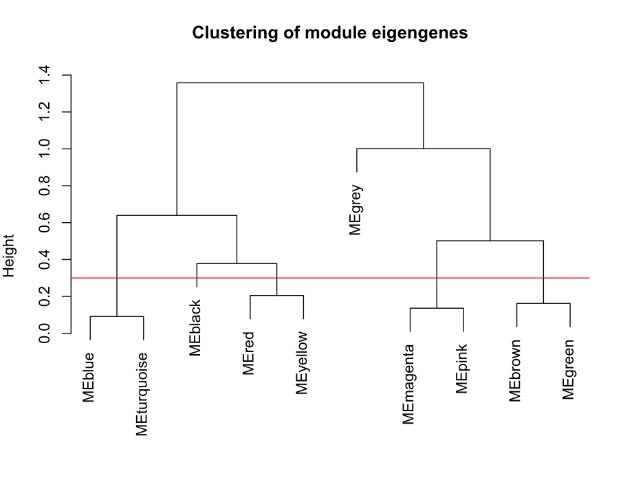
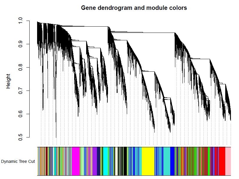
加入模块 minModuleSize = 30 # Module identification using dynamic tree cut: dynamicMods = cutreeDynamic(dendro = geneTree, distM = dissTOM, deepSplit = 2, pamRespectsDendro = FALSE, minClusterSize = minModuleSize); table(dynamicMods) # Convert numeric lables into colors dynamicColors = labels2colors(dynamicMods) table(dynamicColors) # Plot the dendrogram and colors underneath #sizeGrWindow(8,6) pdf(file="5_Dynamic Tree Cut.pdf",width=8,height=6) plotDendroAndColors(geneTree, dynamicColors, "Dynamic Tree Cut", dendroLabels = FALSE, hang = 0.03, addGuide = TRUE, guideHang = 0.05, main = "Gene dendrogram and module colors") dev.off()

合并模块

做出的WGCNA分析中，具有较多的模块，但是在我们后续的分析中，是使用不到这么多的模块，以及模块越多对我们的分析越困难，那么就必须合并模块信息。具体操作如下。

MEList = moduleEigengenes(datExpr, colors = dynamicColors) MEs = MEList$eigengenes # Calculate dissimilarity of module eigengenes MEDiss = 1-cor(MEs); # Cluster module eigengenes METree = hclust(as.dist(MEDiss), method = "average") # Plot the result #sizeGrWindow(7, 6) pdf(file="6_Clustering of module eigengenes.pdf",width=7,height=6) plot(METree, main = "Clustering of module eigengenes", xlab = "", sub = "") MEDissThres = 0.3######剪切高度可修改 # Plot the cut line into the dendrogram abline(h=MEDissThres, col = "red") dev.off()

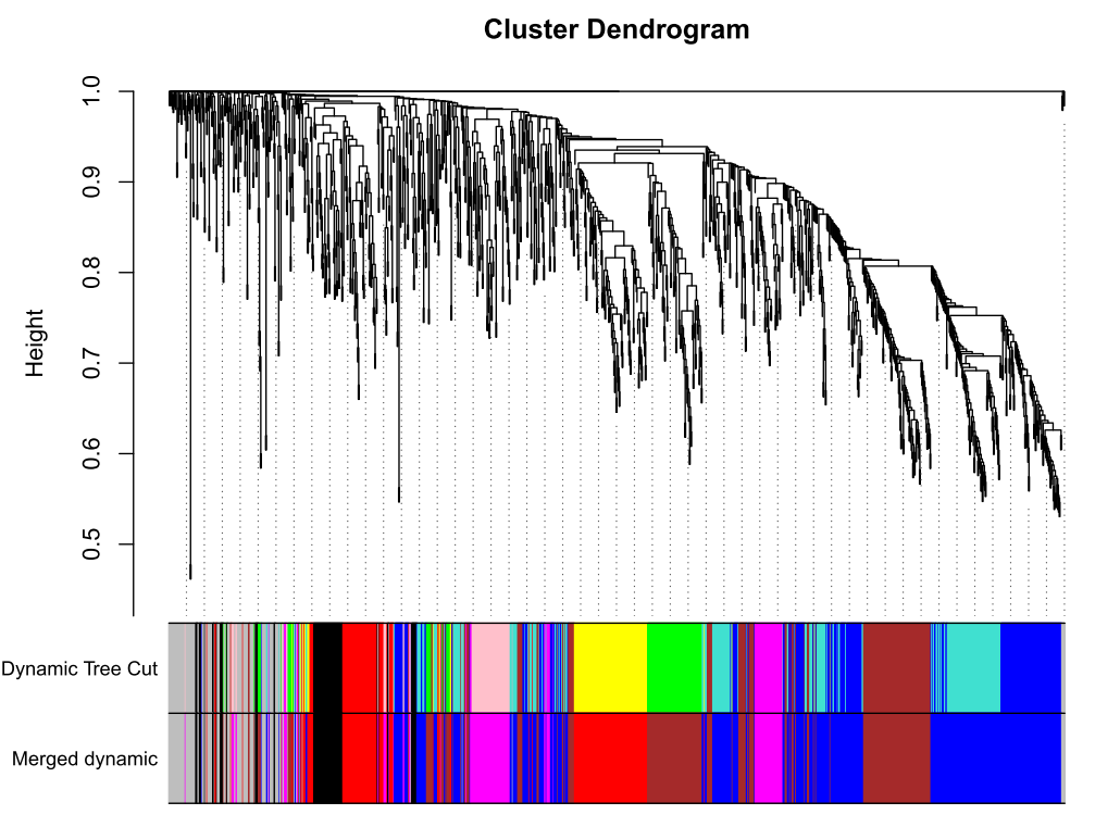
合并及绘图

merge = mergeCloseModules(datExpr, dynamicColors, cutHeight = MEDissThres, verbose = 3) # The merged module colors mergedColors = merge$colors # Eigengenes of the new merged modules: mergedMEs = merge$newMEs table(mergedColors) #输出所有modules color

【本文地址】

WGCNA分析教程五

WGCNA分析教程五

今日新闻

推荐新闻