神经网络的票房预测CNN |
您所在的位置:网站首页 › 预测票房用什么算法 › 神经网络的票房预测CNN |
神经网络的票房预测CNN
|
1、摘要
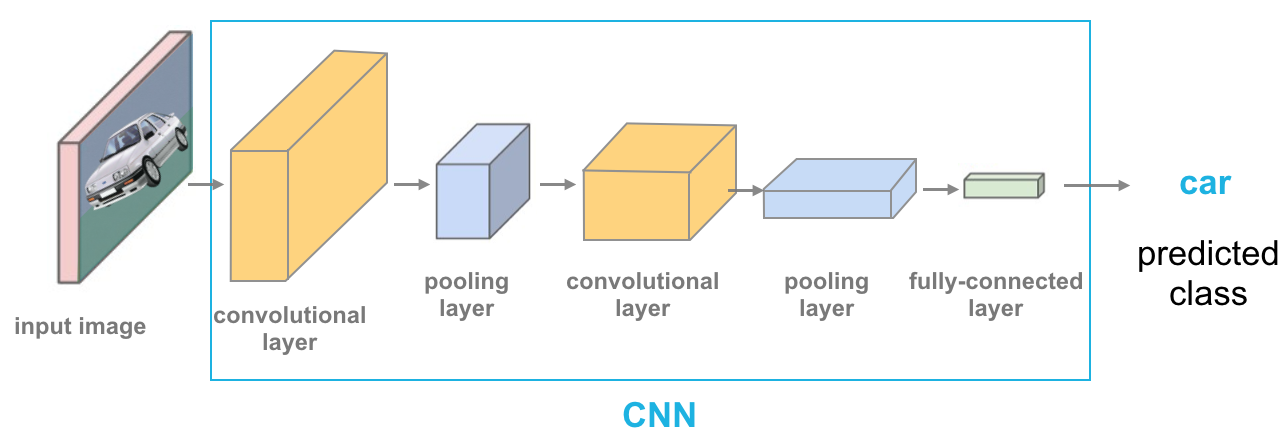
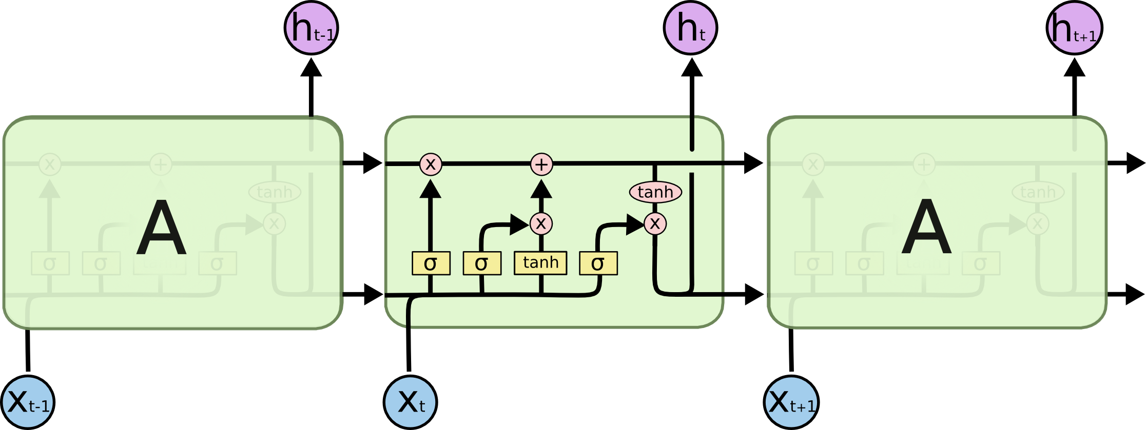
本文主要讲解:神经网络的票房预测,三种实现方式CNN、RNN、LSTM 主要思路: 1、用不少于3种神经网络构建电影票房预测模型,并在同一个数据集上进行训练和预测,对比各个模型的准确率,并可视化。(使用CNN、RNN、LSTM) 2、对数据预处理并对数据进行可视化:分析预算对票房的影响、观众打分对票房影响、流行系数对票房影响、预算和观众打分对票房的影响,电影语言对票房的影响、票房的正态分布。 3、对神经网络结构、多个模型比对、训练过程进行可视化 4、特征分析 2、数据介绍训练的数据集:Kaggle的movie数据集 其中主要特征有: Budget:预算 Revenue:票房 Rating:观众打分 totalVotes:观众打分数量 popularity:流行系数 3、相关技术CNN:卷积神经网络 LSTM:长短期记忆网络,对于长期记忆的时间序列效果比RNN好 此代码的依赖环境如下: numpy==1.19.5 matplotlib==3.5.2 torch==1.9.0 pandas==1.1.5代码输出如下: 在这里插入图片描述 主运行程序入口 import os import warnings from datetime import datetime import matplotlib.pyplot as plt import numpy as np import optuna import pandas as pd import seaborn as sns import torch from sklearn.model_selection import KFold from torch import nn # 这两行代码解决 plt 中文显示的问题 plt.rcParams['font.sans-serif'] = ['SimHei'] plt.rcParams['axes.unicode_minus'] = False # fix random seed 设定随机种子,防止每次训练的结果不一样 def same_seeds(seed): torch.manual_seed(seed) # 固定随机种子(CPU) if torch.cuda.is_available(): # 固定随机种子(GPU) torch.cuda.manual_seed(seed) # 为当前GPU设置 torch.cuda.manual_seed_all(seed) # 为所有GPU设置 np.random.seed(seed) # 保证后续使用random函数时,产生固定的随机数 torch.backends.cudnn.benchmark = False # GPU、网络结构固定,可设置为True torch.backends.cudnn.deterministic = True # 固定网络结构 same_seeds(22) np.random.seed(22) device = torch.device("cuda:0" if torch.cuda.is_available() else "cpu") warnings.filterwarnings("ignore") os.chdir(r'C:\Projects\old\电影数据集多模型对比\data') ''' CNN RNN LSTM 对神经网络结构、多模型对比、训练过程进行可视化 预测值和真实值误差小于0.1,每个模型预测的准确率0.8以上,至少一个0.9 特征分析 ''' # 迭代次数 # epoch_time = 5 # 文中提到的双曲线性单元激活函数 class HLU(nn.Module): def __init__(self): super(HLU, self).__init__() def forward(self, x, alpha=0.15): inputs_m = torch.where(x = 0.0, x, inputs_m * alpha / (1 - inputs_m)) def cnn_model(X_train, y_train, X_val, y_val, X_test): class Model(nn.Module): def __init__(self): super().__init__() self.layer1 = nn.Sequential( nn.Conv1d(X_train.shape[1], 56, 1, 1), nn.BatchNorm1d(num_features=56), HLU(), nn.Dropout(0.29), nn.Conv1d(56, 28, 1, 2), nn.BatchNorm1d(num_features=28), HLU(), nn.Dropout(0.29), nn.Conv1d(28, 14, 1, 2), nn.BatchNorm1d(num_features=14), HLU(), nn.Dropout(0.29), nn.Flatten(), nn.Linear(14, 1) ) def forward(self, x): x = self.layer1(x) return x model = Model() # img = tw.draw_model(model, [56, 198, 1]) # img.save(r'CNN.jpg') # 学习率 learn_rate = 0.2346 loss_function = torch.nn.L1Loss() # 优化器,变量依次为待优化参数。学习率、动量 optim = torch.optim.SGD(model.parameters(), learn_rate, momentum=0.5) # 训练集前固定写法(不写也无妨) model.train() loss_list = [] for epoch in range(41): output = model(X_train) # 计算损失 res_loss = loss_function(y_train, output) # 清零梯度 optim.zero_grad() # 反向传播 res_loss.backward() # 更新参数 optim.step() loss_list.append(res_loss) print(f"训练batch:{i + 1},损失值:{res_loss}") plt.plot(loss_list) plt.title('CNN训练loss变化图') plt.ylabel('mae') plt.xlabel('Epoch') plt.legend(['mae'], loc='best') plt.savefig("CNN训练loss变化图.png", dpi=500, bbox_inches='tight') plt.show() # 测试集固定写法 model.eval() # 测试集不需要梯度下降,加快计算效率 with torch.no_grad(): output = model(X_val) mae = loss_function(y_val, output) val_loss = mae.item() print(f"预测值和真实值误差:{val_loss}") return val_loss def rnn_model(X_train, y_train, X_val, y_val, X_test): plt.figure(1, figsize=(30, 10)) plt.ion() # continuously plot class RNN(nn.Module): def __init__(self): super(RNN, self).__init__() self.rnn = nn.RNN( input_size=1, hidden_size=82, # rnn hidden unit num_layers=1, # number of rnn layer batch_first=True, dropout=0.29 # input & output will has batch size as 1s dimension. e.g. (batch, time_step, input_size) ) self.out = nn.Linear(82, 1) def forward(self, x): r_out, _ = self.rnn(x) r_out = r_out.reshape(-1, 82) r_out = self.out(r_out) return r_out batch_size = 16 rnn = RNN() # img = tw.draw_model(rnn, [1, 83, 1]) # img.save(r'RNN.jpg') rnn.to(device) rnn.train() optimizer = torch.optim.Adam(rnn.parameters(), lr=0.2346) # optimize all cnn parameters loss_function = nn.L1Loss() length = len(X_train) loss_list = [] for step in range(41): for j in range(0, length, batch_size): X_train_batch = X_train[j:j + batch_size] y_train_batch = y_train[j:j + batch_size] X_train_batch = X_train_batch.to(device) y_train_batch = y_train_batch.to(device) y_pred = rnn(X_train_batch) loss = loss_function(y_pred, y_train_batch) optimizer.zero_grad() # clear gradients for this training step loss.backward() # backpropagation, compute gradients optimizer.step() loss_list.append(loss) print(f"训练batch:{step + 1},损失值:{loss}") plt.plot(loss_list) plt.title('RNN训练loss变化图') plt.ylabel('mae') plt.xlabel('Epoch') plt.legend(['mae'], loc='best') plt.savefig("RNN训练loss变化图.png", dpi=500, bbox_inches='tight') plt.show() # test rnn.eval() vl = 0.0 length = len(X_val) with torch.no_grad(): for j in range(0, length, batch_size): X_val_batch = X_val[j:j + batch_size] y_val_batch = y_val[j:j + batch_size] X_val_batch = X_val_batch.to(device) y_val_batch = y_val_batch.to(device) output = rnn(X_val_batch) # 计算损失 mae = loss_function(y_val_batch, output) vl += mae.item() batch_count = len(X_val) // batch_size val_loss = vl / batch_count print(f"预测值和真实值误差:{val_loss}") return val_loss def objective(trial): hidden_size = trial.suggest_int('hidden_size', 60, 100) epoch_time = trial.suggest_int('epoch_time', 33, 55) batch_size = trial.suggest_int('batch_size', 16, 16) dropout = trial.suggest_uniform('dropout', 0.28, 0.3) lr = trial.suggest_uniform('lr', 0.23, 0.25) num_layers = trial.suggest_categorical('num_layers', [1]) print([hidden_size, epoch_time, batch_size, dropout, lr, num_layers]) input_size, hidden_size, num_layers, output_size = 1, hidden_size, num_layers, 1 model = LSTM(input_size, hidden_size, num_layers, output_size, dropout) model = model.to(device) loss_function = nn.L1Loss() X_train_p = pd.read_csv('./X_train.csv') y_train_p = pd.read_csv('./y_train.csv') data = pd.concat([X_train_p, y_train_p], axis=1) data = data[~data.isin([np.nan, np.inf, -np.inf]).any(1)] data.reset_index(inplace=True) X_train_p = data.iloc[:, :-1] y_train_p = pd.DataFrame(data.iloc[:, -1]) k = 2 fold = list(KFold(k, shuffle=True, random_state=random_seed).split(X_train_p)) maes = [] for i, (train, val) in enumerate(fold): X_train = X_train_p.loc[train, :].values y_train = y_train_p.loc[train, :].values X_val = X_train_p.loc[val, :].values y_val = y_train_p.loc[val, :].values.ravel() X_train = torch.FloatTensor(X_train.reshape((X_train.shape[0], X_train.shape[1], 1))) y_train = torch.FloatTensor(y_train.ravel()) X_val = torch.FloatTensor(X_val.reshape((X_val.shape[0], X_val.shape[1], 1))) y_val = torch.FloatTensor(y_val) length = len(X_train) model.train() optimizer = torch.optim.SGD(model.parameters(), lr=lr) for i in range(epoch_time): for j in range(0, length, batch_size): X_train_batch = X_train[j:j + batch_size] y_train_batch = y_train[j:j + batch_size] X_train_batch = X_train_batch.to(device) y_train_batch = y_train_batch.to(device) y_pred = model(X_train_batch) loss = loss_function(y_pred, y_train_batch) optimizer.zero_grad() loss.backward() optimizer.step() model.eval() length = len(X_val) X_val = X_val.to(device) y_val = y_val.to(device) # 测试集不需要梯度下降,加快计算效率 vl = 0.0 with torch.no_grad(): for j in range(0, length, batch_size): X_val_batch = X_val[j:j + batch_size] y_val_batch = y_val[j:j + batch_size] X_val_batch = X_val_batch.to(device) y_val_batch = y_val_batch.to(device) output = model(X_val_batch) # 计算损失 mae = loss_function(y_val_batch, output) vl += mae.item() batch_count = len(X_val) // batch_size val_loss = vl / batch_count maes.append(val_loss) mae = np.array(maes).mean() return mae X_train_p = pd.read_csv('./X_train.csv') X_test = pd.read_csv('./X_test.csv') y_train_p = pd.read_csv('./y_train.csv') data = pd.concat([X_train_p, y_train_p], axis=1) data = data[~data.isin([np.nan, np.inf, -np.inf]).any(1)] data.reset_index(inplace=True) X_train_p = data.iloc[:, :-1] y_train_p = pd.DataFrame(data.iloc[:, -1]) random_seed = 2019 k = 2 fold = list(KFold(k, shuffle=True, random_state=random_seed).split(X_train_p)) np.random.seed(random_seed) for i, (train, val) in enumerate(fold): print(i + 1, "fold") X_train = X_train_p.loc[train, :].values y_train = y_train_p.loc[train, :].values X_val = X_train_p.loc[val, :].values y_val = y_train_p.loc[val, :].values.ravel() mean_y_val = y_val.mean() X_train = torch.FloatTensor(X_train.reshape((X_train.shape[0], X_train.shape[1], 1))) y_train = torch.FloatTensor(y_train.ravel()) X_val = torch.FloatTensor(X_val.reshape((X_val.shape[0], X_val.shape[1], 1))) y_val = torch.FloatTensor(y_val) # """ cnn_model start = datetime.now() cnn_mae = cnn_model(X_train, y_train, X_val, y_val, X_test) print("cnn_model mae ", "{0:.5f}".format(cnn_mae), '(' + str(int((datetime.now() - start).seconds)) + 's)') cnn_acc = round(1 - cnn_mae / mean_y_val, 3) print('cnn_model 准确率:', cnn_acc) # # # # # """ rnn_model start = datetime.now() rnn_mae = rnn_model(X_train, y_train, X_val, y_val, X_test) print("rnn_model mae.", "{0:.5f}".format(rnn_mae), '(' + str(int((datetime.now() - start).seconds)) + 's)') rnn_acc = round(1 - rnn_mae / mean_y_val, 3) print('rnn_model 准确率:', rnn_acc) # """ lstm_model class LSTM(nn.Module): def __init__(self, input_size, hidden_size, num_layers, output_size, dropout): super().__init__() self.input_size = input_size self.hidden_size = hidden_size self.num_layers = num_layers self.output_size = output_size self.lstm = nn.LSTM(self.input_size, self.hidden_size, self.num_layers, dropout=dropout, batch_first=True) self.linear = nn.Linear(self.hidden_size, self.output_size) def forward(self, input_seq): x, _ = self.lstm(input_seq) x = x.reshape(-1, self.hidden_size) pred = self.linear(x) return pred """ Run optimize. Set n_trials and/or timeout (in sec) for optimization by Optuna """ study = optuna.create_study(direction='minimize') study.optimize(objective, n_trials=11) print('Best trial number: ', study.best_trial.number) print('Best value:', study.best_trial.value) print('Best parameters: \n', study.best_trial.params) parameters = study.best_trial.params # parameters = {'hidden_size': 82, 'epoch_time': 41, 'batch_size': 16, 'dropout': 0.2904, 'lr': 0.2346, # 'num_layers': 1} hidden_size = parameters['hidden_size'] batch_size = parameters['batch_size'] dropout = parameters['dropout'] lr = parameters['lr'] num_layers = parameters['num_layers'] epoch_time = parameters['epoch_time'] input_size, hidden_size, num_layers, output_size = 1, hidden_size, num_layers, 1 model = LSTM(input_size, hidden_size, num_layers, output_size, dropout) # img = tw.draw_model(model, [1, 82, 1]) # img.save(r'LSTM.jpg') model = model.to(device) loss_function = nn.L1Loss().to(device) optimizer = torch.optim.Adam(model.parameters(), lr=lr) model.train() loss_list = [] for i in range(epoch_time): for j in range(0, len(X_train), batch_size): X_train_batch = X_train[j:j + batch_size] y_train_batch = y_train[j:j + batch_size] X_train_batch = X_train_batch.to(device) y_train_batch = y_train_batch.to(device) y_pred = model(X_train_batch) loss = loss_function(y_pred, y_train_batch) optimizer.zero_grad() loss.backward() optimizer.step() loss_list.append(loss) print(f"训练batch:{i + 1},损失值:{loss}") plt.plot(loss_list) plt.title('LSTM训练loss变化图') plt.ylabel('mae') plt.xlabel('Epoch') plt.legend(['mae'], loc='best') plt.savefig("LSTM训练loss变化图.png", dpi=500, bbox_inches='tight') plt.show() model.eval() length = len(X_val) X_val = X_val.to(device) y_val = y_val.to(device) # 测试集不需要梯度下降,加快计算效率 vl = 0.0 with torch.no_grad(): for j in range(0, length, batch_size): X_val_batch = X_val[j:j + batch_size] y_val_batch = y_val[j:j + batch_size] X_val_batch = X_val_batch.to(device) y_val_batch = y_val_batch.to(device) output = model(X_val_batch) # 计算损失 mae = loss_function(y_val_batch, output) vl += mae.item() batch_count = len(X_val) // batch_size lstm_mae = vl / batch_count print(f"预测值和真实值误差:{lstm_mae}") lstm_acc = round(1 - lstm_mae / mean_y_val, 3) print('lstm_model 准确率:', lstm_acc) def labels(ax): for p in ax.patches: width = p.get_width() # get bar length ax.text(width, # set the text at 1 unit right of the bar p.get_y() + p.get_height() / 2, # get Y coordinate + X coordinate / 2 '{:1.3f}'.format(width), # set variable to display, 2 decimals ha='left', # horizontal alignment va='center') # vertical alignment # 模型比较 compare = pd.DataFrame({"Model": ["CNN", "RNN", "LSTM"], "MAE": [cnn_mae, rnn_mae, lstm_mae], "Accuracy": [cnn_acc, rnn_acc, lstm_acc]}) plt.figure(figsize=(14, 14)) plt.subplot(211) compare = compare.sort_values(by="MAE", ascending=False) ax = sns.barplot(x="MAE", y="Model", data=compare, palette="Blues_d") labels(ax) plt.subplot(212) compare = compare.sort_values(by="Accuracy", ascending=False) ax = sns.barplot(x="Accuracy", y="Model", data=compare, palette="Blues_d") labels(ax) plt.show()完整数据和代码链接: 神经网络的票房预测CNN-RNN-LSTM |
 RNN:循环神经网络
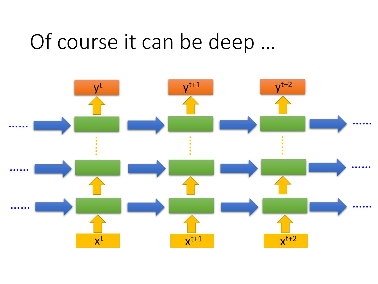


【本文地址】
今日新闻 |
推荐新闻 |