基于MATLAB的硬约束轨迹优化算法代码学习 |
您所在的位置:网站首页 › 路径规划算法工程师考试题及答案 › 基于MATLAB的硬约束轨迹优化算法代码学习 |
基于MATLAB的硬约束轨迹优化算法代码学习
|
基于MATLAB的硬约束轨迹优化算法代码学习
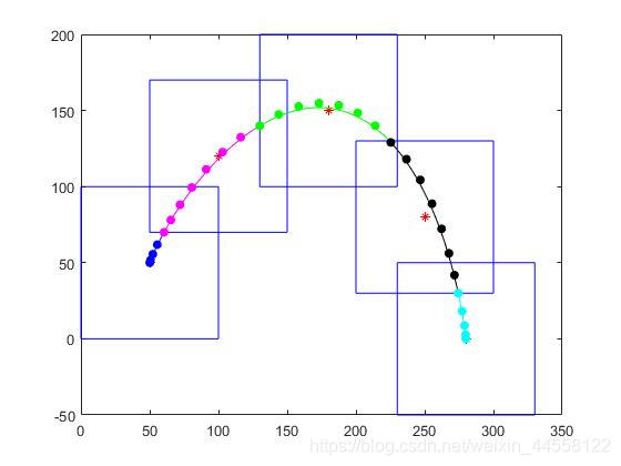
0.结果展示1.hw_6.m2.getQM.m3.getM.m4.getAbeq.m5.getAbieq.m6.参考引用
本文是在学习路径规划算法中的一篇学习记录,将整个代码进行了详细的梳理,方便后来者参考学习.代码需要和理论部分结合起来看更容易理解,理论部分:
《软约束和硬约束下的轨迹优化-学习记录 》.
(代码注释中英夹杂,英文注释是原来作者的注释,中文注释是本人后来添加的) 0.结果展示
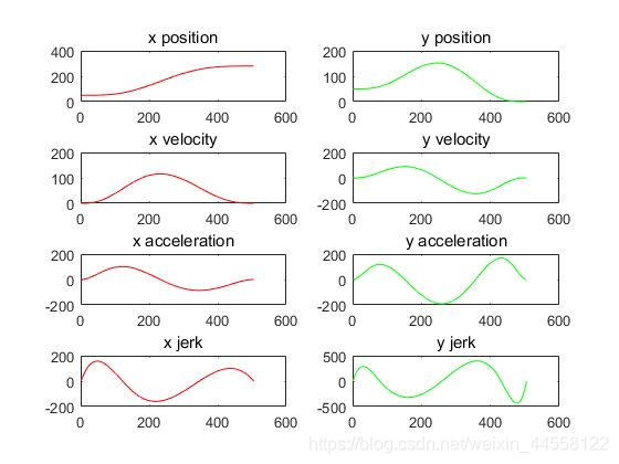
这部分是主函数部分,主要包括计算和画图。 clc;clear;close all % 设定v、a、j的限制 v_max = 400; a_max = 400; j_max = 100000; color = ['r', 'b', 'm', 'g', 'k', 'c', 'c']; %% specify the center points of the flight corridor and the region of corridor % 设定飞行走廊中心点 path = [50, 50; 100, 120; 180, 150; 250, 80; 280, 0]; % 设定飞行走廊x、y轴的边界 x_length = 100; y_length = 100; n_order = 7; % 8 control points n_order = 2*d_order - 1 % 7 = 2*4 -1 minimal snap defferenational order is 4, p,v,a,j must be % continuous and differentialble, it can provide 2*4 euqtions, so the % variables can be up to 8 n_seg = size(path, 1); % 设定每个走廊的相关信息 corridor = zeros(4, n_seg); for i = 1:n_seg % 对于每一列而言,前面两个是坐标,后面两个是走廊长宽 corridor(:, i) = [path(i, 1), path(i, 2), x_length/2.0, y_length/2.0]'; end %% specify ts for each segment %每一段轨迹的时间分配为1s ts = zeros(n_seg, 1); for i = 1:n_seg ts(i,1) = 1; end % 独立对各轴求解 poly_coef_x = MinimumSnapCorridorBezierSolver(1, path(:, 1), corridor, ts, n_seg, n_order, v_max, a_max, j_max); disp("x axle solved!") poly_coef_y = MinimumSnapCorridorBezierSolver(2, path(:, 2), corridor, ts, n_seg, n_order, v_max, a_max, j_max); disp("y axle solved!") %% display the trajectory and cooridor plot(path(:,1), path(:,2), '*r'); hold on; for i = 1:n_seg plot_rect([corridor(1,i);corridor(2,i)], corridor(3, i), corridor(4,i));hold on; end hold on; %% ##################################################### % STEP 4: draw bezier curve x_pos = [];y_pos = []; x_vel = [];y_vel = []; x_acc = [];y_acc = []; x_jerk = [];y_jerk = []; idx = 1; for j = 1:n_seg start_pos_id = idx; for t = 0:0.01:1 x_pos(idx) = 0.0;y_pos(idx) = 0.0; x_vel(idx) = 0.0;y_vel(idx) = 0.0; x_acc(idx) = 0.0;y_acc(idx) = 0.0; x_jerk(idx) = 0.0;y_jerk(idx) = 0.0; for i = 0:n_order start_idx = (j-1)*(n_order+1)+i; basis_p = nchoosek(n_order, i) * t^i * (1-t)^(n_order-i); x_pos(idx) = x_pos(idx) + poly_coef_x(start_idx+1)*basis_p*ts(j); y_pos(idx) = y_pos(idx) + poly_coef_y(start_idx+1)*basis_p*ts(j); if i < n_order basis_v = nchoosek(n_order-1, i) * t^i *(1-t)^(n_order-1-i); x_vel(idx) = x_vel(idx) + (n_order+1) * (poly_coef_x(start_idx+2)-poly_coef_x(start_idx+1))*basis_v; y_vel(idx) = y_vel(idx) + (n_order+1) * (poly_coef_y(start_idx+2)-poly_coef_y(start_idx+1))*basis_v; end if i < n_order-1 basis_a = nchoosek(n_order-2, i) * t^i *(1-t)^(n_order-2-i); x_acc(idx) = x_acc(idx) + (n_order+1) * n_order * (poly_coef_x(start_idx+3) - 2*poly_coef_x(start_idx+2) + poly_coef_x(start_idx+1))*basis_a/ts(j); y_acc(idx) = y_acc(idx) + (n_order+1) * n_order * (poly_coef_y(start_idx+3) - 2*poly_coef_y(start_idx+2) + poly_coef_y(start_idx+1))*basis_a/ts(j); end if i < n_order-2 basis_j = nchoosek(n_order-3, i) * t^i *(1-t)^(n_order-3-i); x_jerk(idx) = x_jerk(idx) + (n_order+1) * n_order * (n_order-1) * ... (poly_coef_x(start_idx+4) - 3*poly_coef_x(start_idx+3) + 3*poly_coef_x(start_idx+2) - poly_coef_x(start_idx+1)) * basis_j/ts(j)^2; y_jerk(idx) = y_jerk(idx) + (n_order+1) * n_order * (n_order-1) * ... (poly_coef_y(start_idx+4) - 3*poly_coef_y(start_idx+3) + 3*poly_coef_y(start_idx+2) - poly_coef_y(start_idx+1)) * basis_j/ts(j)^2; end end idx = idx + 1; end end_pos_id = idx - 1; scatter(ts(j)*poly_coef_x((j-1)*(n_order+1)+1:(j-1)*(n_order+1)+1+n_order), ts(j)*poly_coef_y((j-1)*(n_order+1)+1:(j-1)*(n_order+1)+1+n_order), 'filled',color(mod(j,7)+1),'LineWidth', 5);hold on; plot(x_pos(start_pos_id:end_pos_id), y_pos(start_pos_id:end_pos_id), color(mod(j,7)+1));hold on; end figure(2) subplot(4,2,1) plot(x_pos, 'Color', 'r');title('x position'); subplot(4,2,2) plot(y_pos, 'Color', 'g');title('y position'); subplot(4,2,3) plot(x_vel, 'Color', 'r');title('x velocity'); subplot(4,2,4) plot(y_vel, 'Color', 'g');title('y velocity'); subplot(4,2,5) plot(x_acc, 'Color', 'r');title('x acceleration'); subplot(4,2,6) plot(y_acc, 'Color', 'g');title('y acceleration'); subplot(4,2,7) plot(x_jerk, 'Color', 'r');title('x jerk'); subplot(4,2,8) plot(y_jerk, 'Color', 'g');title('y jerk'); function poly_coef = MinimumSnapCorridorBezierSolver(axis, waypoints, corridor, ts, n_seg, n_order, v_max, a_max, j_max) start_cond = [waypoints(1), 0, 0, 0]; end_cond = [waypoints(end), 0, 0, 0]; %% ##################################################### % STEP 1: compute Q_0 of c'Q_0c [Q, M] = getQM(n_seg, n_order, ts); Q_0 = M'*Q*M; % 返回和Q矩阵距离最近的一个对称正定(Symmetric Positive Definite)矩阵Q'. % 目的是在把目标函数微调为一个凸函数,保证得到的解为全局最优解. Q_0 = nearestSPD(Q_0); %% ##################################################### % STEP 2: get Aeq and beq [Aeq, beq] = getAbeq(n_seg, n_order, ts, start_cond, end_cond); %% ##################################################### % STEP 3: get corridor_range, Aieq and bieq % STEP 3.1: get corridor_range of x-axis or y-axis, % you can define corridor_range as [p1_min, p1_max; % p2_min, p2_max; % ..., % pn_min, pn_max ]; corridor_range = zeros(n_seg,2); for k = 1:n_seg % 横坐标/纵坐标减去、加上corridor宽度得到x/y轴边界 corridor_range(k,:) = [corridor(axis,k) - corridor(axis+2,k), corridor(axis,k) + corridor(axis+2,k)]; end % STEP 3.2: get Aieq and bieq [Aieq, bieq] = getAbieq(n_seg, n_order, corridor_range, ts, v_max, a_max, j_max); f = zeros(size(Q_0,1),1); % quadprog函数参数介绍:https://blog.csdn.net/tianzy16/article/details/87916128 poly_coef = quadprog(Q_0,f,Aieq, bieq, Aeq, beq); end function plot_rect(center, x_r, y_r) p1 = center+[-x_r;-y_r]; p2 = center+[-x_r;y_r]; p3 = center+[x_r;y_r]; p4 = center+[x_r;-y_r]; plot_line(p1,p2); plot_line(p2,p3); plot_line(p3,p4); plot_line(p4,p1); end function plot_line(p1,p2) a = [p1(:),p2(:)]; plot(a(1,:),a(2,:),'b'); end 2.getQM.m获得Q矩阵。 function [Q, M] = getQM(n_seg, n_order, ts) Q = []; M = []; % 因为我们将时间映射到[0,1]区间内,所以这个getM函数可以固化下来 M_k = getM(n_order); % d_order = 4; for k = 1:n_seg %##################################################### % STEP 2.1 calculate Q_k of the k-th segment % Q_k = []; fac = @(x) x*(x-1)*(x-2)*(x-3); Q_k = zeros(n_order+1,n_order+1); for i = 0:n_order for j = 0:n_order if (i < 4) || (j < 4) continue; else % 也即 i!/(i-4)! * j!/(j-4)! * 1/(i+j-7) * t^(j+i-7) Q_k(i+1,j+1) = fac(i) * fac(j)/(i + j - 7) * ts(k)^(j+i-7); end end end Q = blkdiag(Q, Q_k); M = blkdiag(M, M_k); end end 3.getM.m获得M矩阵。 function M = getM(n_order) if n_order == 3 M = [ 1 0 0 0; -3 3 0 0; 3 -6 3 0; -1 3 -3 1]; elseif n_order == 4 % Degree D = 4 M = [1 0 0 0 0 ; -4 4 0 0 0 ; 6 -12 6 0 0 ; -4 12 -12 4 0 ; 1 -4 6 -4 1 ]; elseif n_order == 5 % Degree D = 5 M = [1 0 0 0 0 0 -5 5 0 0 0 0; 10 -20 10 0 0 0; -10 30 -30 10 0 0; 5 -20 30 -20 5 0; -1 5 -10 10 -5 1 ]; elseif n_order == 6 % Degree D = 6 M = [1 0 0 0 0 0 0; -6 6 0 0 0 0 0; 15 -30 15 0 0 0 0; -20 60 -60 20 0 0 0; 15 -60 90 -60 15 0 0; -6 30 -60 60 -30 6 0; 1 -6 15 -20 15 -6 1 ]; elseif n_order == 7 % Degree D = 7 M = [ 1 0 0 0 0 0 0 0; -7 7 0 0 0 0 0 0; 21 -42 21 0 0 0 0 0 -35 105 -105 35 0 0 0 0; 35 -140 210 -140 35 0 0 0; -21 105 -210 210 -105 21 0 0; 7 -42 105 -140 105 -42 7 0; -1 7 -21 35 -35 21 -7 1]; elseif n_order == 8 % Degree D = 8 M = [ 1 0 0 0 0 0 0 0 0 ; -8 8 0 0 0 0 0 0 0; 28 -56 28 0 0 0 0 0 0; -56 168 -168 56 0 0 0 0 0; 70 -280 420 -280 70 0 0 0 0; -56 280 -560 560 -280 56 0 0 0; 28 -168 420 -560 420 -168 28 0 0; -8 56 -168 280 -280 168 -56 8 0; 1 -8 28 -56 70 -56 28 -8 1]; elseif n_order == 9 % Degree D = 9 M = [ 1 0 0 0 0 0 0 0 0 0; -9 9 0 0 0 0 0 0 0 0; 36 -72 36 0 0 0 0 0 0 0; -84 252 -252 84 0 0 0 0 0 0; 126 -504 756 -504 126 0 0 0 0 0; -126 630 -1260 1260 -630 126 0 0 0 0; 84 -504 1260 -1680 1260 -504 84 0 0 0; -36 252 -756 1260 -1260 756 -252 36 0 0; 9 -72 252 -504 630 -504 252 -72 9 0; -1 9 -36 84 -126 126 -84 36 -9 1]; end end 4.getAbeq.m获得线性等式约束的系数矩阵和右端向量。 function [Aeq, beq] = getAbeq(n_seg, n_order, ts, start_cond, end_cond) n_all_poly = n_seg*(n_order+1); % 所有控制点多项式系数总和 %##################################################### % STEP 2.1 p,v,a,j constraint in start Aeq_start = zeros(4, n_all_poly); % Ascending order Aeq_start(1,1:4) = [1,0,0,0] * ts(1)^(1);% c0 Aeq_start(2,1:4) = n_order * [-1,1,0,0] * ts(1)^(0);% c'0 = n*(c1 - c0) Aeq_start(3,1:4) = n_order * (n_order-1) * [1,-2,1,0] * ts(1)^(-1);% c''0 = n*(n-1)*(c2 -2*c1 +c0) Aeq_start(4,1:4) = n_order * (n_order-1) * (n_order-2) * [1,-3,3,-1] * ts(1)^(-2);% c''0 = n*(n-1)*(n-2)*(c3 - 3*c2 + 3*c1 - c0) beq_start = start_cond'; %##################################################### % STEP 2.2 p,v,a,j constraint in end Aeq_end = zeros(4, n_all_poly); % Descending order Aeq_end(1,end-3:end) = [1,0,0,0] * ts(end)^(1);% cn Aeq_end(2,end-3:end) = n_order * [-1,1,0,0] * ts(end)^(0);% c'n-1 = n*(cn -cn-1) Aeq_end(3,end-3:end) = n_order * (n_order-1) * [1,-2,1,0] * ts(end)^(-1);% c''n-2 = n^2*(n-1)*(cn - 2*cn-1 + cn-2) Aeq_end(4,end-3:end) = n_order * (n_order-1) * (n_order-2) * [1,-3,3,-1] * ts(end)^(-2);% c''n-3 = n*(n-1)*(n-2)*(cn - 3*cn-1 + 3*cn-2 - c0) beq_end = end_cond'; %##################################################### % STEP 2.3 position continuity constrain between 2 segments Aeq_con_p = zeros(n_seg-1, n_all_poly); % n_seg-1:轨迹段数 d = 0; % 导数阶数 for k = 1:n_seg-1 Aeq_con_p(k,k*(n_order+1)) = 1 * ts(k)^(1-d); Aeq_con_p(k,k*(n_order+1)+1) = -1 * ts(k+1)^(1-d); end beq_con_p = zeros(n_seg-1,1); %##################################################### % STEP 2.4 velocity continuity constrain between 2 segments Aeq_con_v = zeros(n_seg-1, n_all_poly); d = 1; for k = 1:n_seg-1 % (c(n))- c(n-1)) segment 1 + (-c1 + c0) segment 2 Aeq_con_v(k,k*(n_order+1)-1:k*(n_order+1)) = [-1, 1] * ts(k)^(1-d); Aeq_con_v(k,k*(n_order+1)+1:k*(n_order+1)+2) = [1, -1] * ts(k+1)^(1-d); end beq_con_v = zeros(n_seg-1,1); %##################################################### % STEP 2.5 acceleration continuity constrain between 2 segments Aeq_con_a = zeros(n_seg-1, n_all_poly); d = 2; for k = 1:n_seg-1 % (c(n))- 2*c(n-1) + c(n-2)) segment 1 + (-c2 + 2*c1 - c0) segment 2 Aeq_con_a(k,k*(n_order+1)-2:k*(n_order+1)) = [1, -2, 1] * ts(k)^(1-d); Aeq_con_a(k,k*(n_order+1)+1:k*(n_order+1)+3) = [-1, 2, -1] * ts(k+1)^(1-d); end beq_con_a = zeros(n_seg-1,1); %##################################################### % STEP 2.6 jerk continuity constrain between 2 segments Aeq_con_j = zeros(n_seg-1, n_all_poly); d = 3; for k = 1:n_seg-1 % (c(n))- 3*c(n-1) + 3*c(n-2) - c(n-3)) segment 1 + (-c3 + 3*c2 - 3*c1 + c0) segment 2 Aeq_con_j(k,k*(n_order+1)-3:k*(n_order+1)) = [1, -3, 3, -1] * ts(k)^(1-d); Aeq_con_j(k,k*(n_order+1)+1:k*(n_order+1)+4) = [-1, 3, -3, 1] * ts(k+1)^(1-d); end beq_con_j = zeros(n_seg-1,1); %##################################################### % combine all components to form Aeq and beq Aeq_con = [Aeq_con_p; Aeq_con_v; Aeq_con_a; Aeq_con_j]; beq_con = [beq_con_p; beq_con_v; beq_con_a; beq_con_j]; Aeq = [Aeq_start; Aeq_end; Aeq_con]; beq = [beq_start; beq_end; beq_con]; end 5.getAbieq.m获得线性不等式约束的系数矩阵和右端向量。 function [Aieq, bieq] = getAbieq(n_seg, n_order, corridor_range, ts, v_max, a_max, j_max) n_all_poly = n_seg*(n_order+1); %##################################################### % STEP 3.2.1 p constraint % 安全性约束 coeff_p = ones(n_all_poly,1); bieq_p = []; for k = 1:n_seg % max % 这个没有完全理解为什么要这么构造? coeff_p(1 + (k-1)*(n_order+1):k*(n_order+1)) = coeff_p(1 + (k-1)*(n_order+1):k*(n_order+1)) * ts(k)^(1); % 放入上边界 bieq_p = [bieq_p;ones(n_order+1,1)*corridor_range(k,2)]; end for k = 1:n_seg % -min % 放入下边界 bieq_p = [bieq_p;ones(n_order+1,1)*corridor_range(k,1)*(-1)]; end Aieq_p = diag(coeff_p,0); Aieq_p = [Aieq_p;-Aieq_p]; %##################################################### % STEP 3.2.2 v constraint % 动力学约束: v n_ctr = n_order; % the number of control posints after first deferention: n_order n_eq = n_ctr*n_seg*2; % number of equations (max and min constraints) Aieq_v = zeros(n_eq/2,n_all_poly); for k = 1:n_seg for n = 1:n_ctr index_col = k*(n_order+1)-1; index_row = n+(k-1)*n_ctr; Aieq_v(index_row,index_col:index_col+1) = n_order * [-1, 1] * ts(k)^(0); end end Aieq_v = [Aieq_v;-Aieq_v]; bieq_v = ones(n_eq,1)* v_max; % bieq_v = ones(n_eq/2,1)* v_max; %##################################################### % STEP 3.2.3 a constraint % 动力学约束: a n_ctr = n_order-1; % the number of control posints after second deferention: n_order - 1 n_eq = n_ctr*n_seg*2; % number of equations (max and min constraints) Aieq_a = zeros(n_eq/2, n_all_poly); for k = 1:n_seg for n = 1:n_ctr index_col = k*(n_order+1)-2; index_row = n+(k-1)*n_ctr; Aieq_a(index_row,index_col:index_col+2) = n_order * (n_order-1) * [1, -2, 1] * ts(k)^(-1); end end Aieq_a = [Aieq_a;-Aieq_a]; bieq_a = ones(n_eq,1)*a_max; % bieq_a = ones(n_eq/2,1)*a_max; % STEP 3.2.4 j constraint n_ctr = n_order-2; % the number of control posints after third deferention: n_order - 2 n_eq = n_ctr*n_seg*2; % number of equations (max and min constraints) Aieq_j = zeros(n_eq/2, n_all_poly); for k = 1:n_seg for n = 1:n_ctr index_col = k*(n_order+1)-3; index_row = n+(k-1)*n_ctr; Aieq_j(index_row,index_col:index_col+3) = n_order * (n_order-1) * (n_order-2) * [1, -3, 3, -1] * ts(k)^(-2); end end Aieq_j = [Aieq_j;-Aieq_j]; bieq_j = ones(n_eq,1)*j_max; %##################################################### % combine all components to form Aieq and bieq Aieq = [Aieq_p; Aieq_v; Aieq_a; Aieq_j]; bieq = [bieq_p; bieq_v; bieq_a; bieq_j]; % Aieq = Aieq_p; % bieq = bieq_p; end 6.参考引用1.理论:深蓝学院; 2.代码:https://github.com/KailinTong/Motion-Planning-for-Mobile-Robots/tree/master/hw_6 |
【本文地址】
今日新闻 |
推荐新闻 |