【Python】精选30张炫酷的动态交互式图表，Pandas一键生成，通俗易懂

您所在的位置：网站首页 › 航班动态图表大全 › 【Python】精选30张炫酷的动态交互式图表，Pandas一键生成，通俗易懂

【Python】精选30张炫酷的动态交互式图表，Pandas一键生成，通俗易懂

2024-06-13 21:38| 来源: 网络整理| 查看: 265

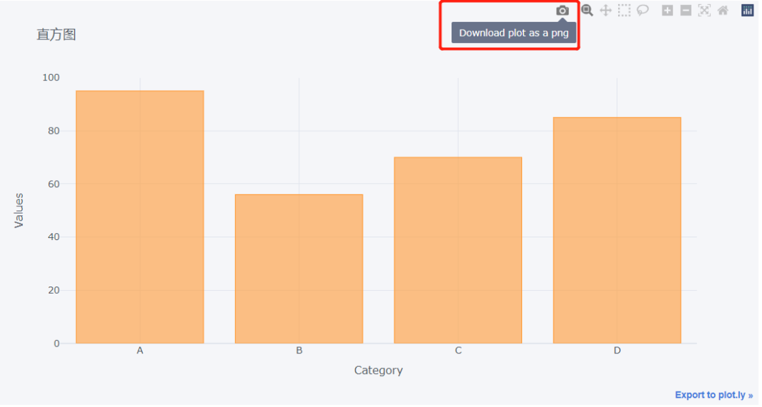
今天小编来讲一下如何用一行代码在DataFrame数据集当中生成炫酷的动态交互式的图表，我们先来介绍一下这次需要用到的模块cufflinks

就像是seaborn封装了matplotlib一样，cufflinks也在plotly上面做了进一步的包装及优化，方法统一、参数配置简单，对于DataFrame数据集而言也可以方便灵活的绘图，而这次我们要绘制的图表包括

折线图

面积图

散点图

柱状图

直方图

箱型图

热力图

3D 散点图/3D 气泡图

趋势图

饼图

K线图

多个子图相拼合

模块的安装

涉及到安装，直接pip install即可

pip install cufflinks 导入模块，并查看相关的配置

我们导入该模块，看一下目前的版本是在多少

cf.__version__

output

'0.17.3'

目前该模块的版本已经到了0.17.3，也是最新的版本，然后我们最新版本支持可以绘制的图表有哪些

cf.help()

output

Use 'cufflinks.help(figure)' to see the list of available parameters for the given figure. Use 'DataFrame.iplot(kind=figure)' to plot the respective figure Figures: bar box bubble bubble3d candle choroplet distplot .......

从上面的输出我们可以看到，绘制图表大致的语法是df.iplot(kind=图表名称)而如何我们想要查看某个特定图表绘制时候的参数，例如柱状图bar参数有哪些，可以这么做

cf.help('bar') 柱状图

我们先来看一下直方图图表的绘制，首先来创建一个数据集用于图表的绘制

df2 = pd.DataFrame({'Category':['A','B','C','D'], 'Values':[95,56,70,85]}) df2

output

Category Values 0 A 95 1 B 56 2 C 70 3 D 85

然后我们来绘制直方图

df2.iplot(kind='bar',x='Category',y='Values', xTitle = "Category",yTitle = "Values", title = "直方图")

output

其中的x参数上面填的是x轴上面对应的变量名，而y参数填的是y轴上面对应的变量名，我们可以将绘制的图表以png的格式下载下来，

同时我们也还可以对绘制的图表放大查看，

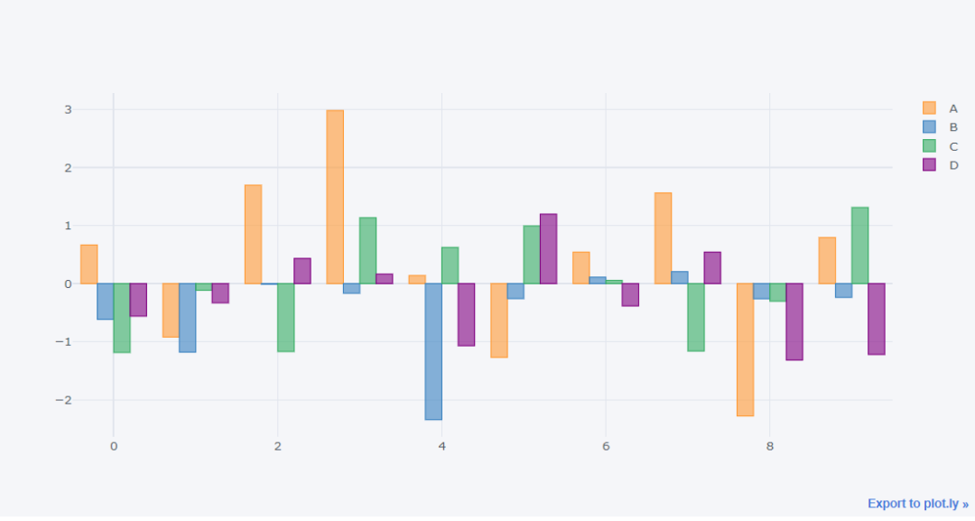
我们再来看一下下面这组数据

df = pd.DataFrame(np.random.randn(100,4),columns='A B C D'.split()) df.head()

output

A B C D 0 0.612403 -0.029236 -0.595502 0.027722 1 1.167609 1.528045 -0.498168 -0.221060 2 -1.338883 -0.732692 0.935410 0.338740 3 1.662209 0.269750 -1.026117 -0.858472 4 1.387077 -0.839192 -0.562382 -0.989672

我们来绘制直方图的图表

df.head(10).iplot('bar')

output

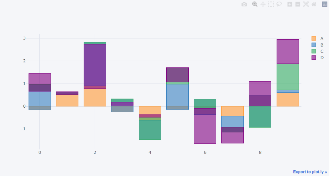
我们也可以来绘制“堆叠式”的直方图

df.head(10).iplot(kind='bar',barmode='stack')

output

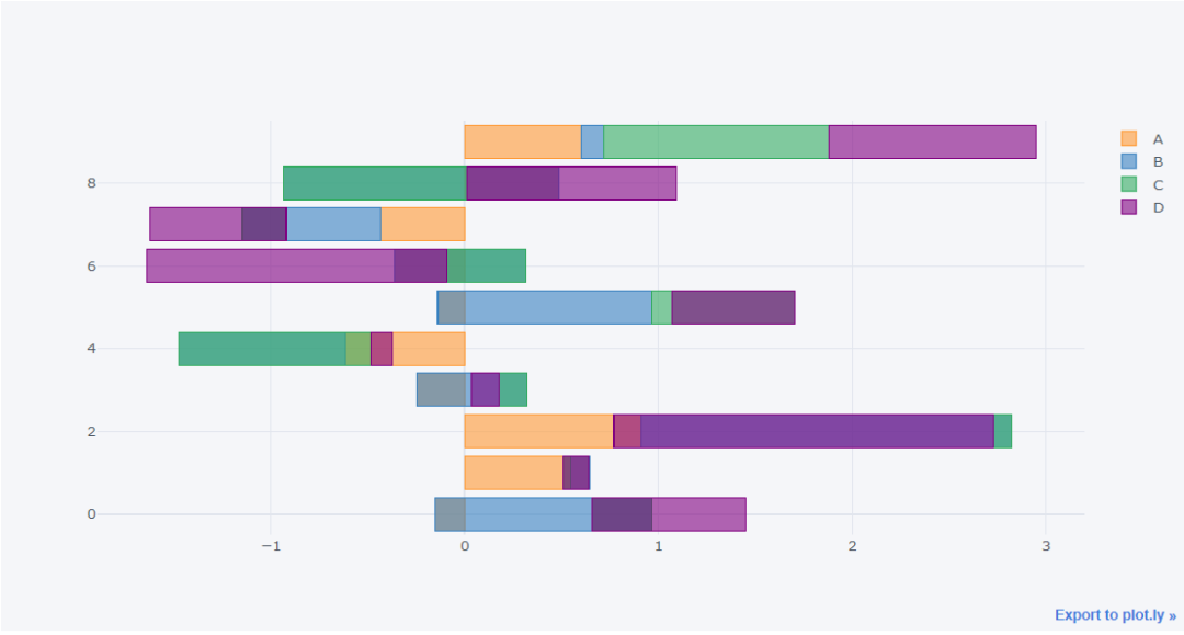
那么同样地，我们也可以将直方图横过来来绘制

df.head(10).iplot(kind='barh',barmode='stack')

output

折线图

下面我们来看一下折线图的绘制，我们首先针对上面的df数据集各列做一个累加

df3 = df.cumsum()

然后我们来绘制折线图

df3.iplot()

output

当然你也可以筛选出当中的几列然后来进行绘制，效果如下

df3[["A", "B"]].iplot()

output

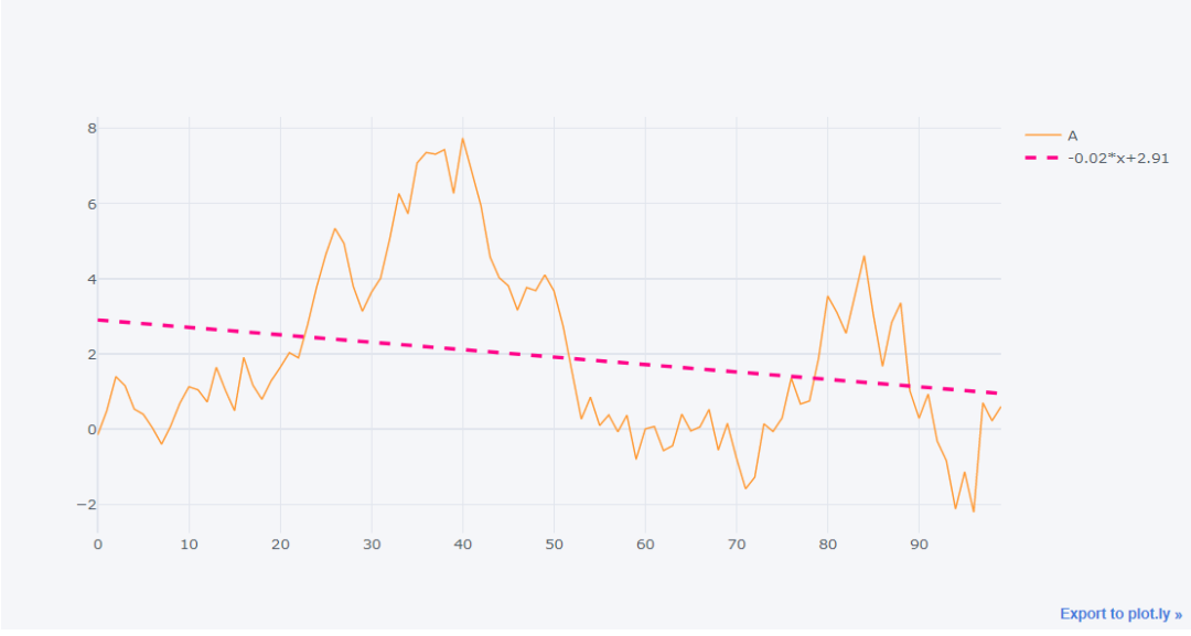
我们也可以给折线图画一条拟合其走势的直线，

df3['A'].iplot(bestfit = True,bestfit_colors=['pink'])

output

这里我们着重来介绍一个iplot()方法里面常用的参数

kind:图表类型，默认的是scatter，散点类型，可供选择的类型还有bar(直方图)、box(箱型图)、heatmap(热力图)等等

theme: 布局主题，可以通过cf.getThemes()来查看主要有哪些

title: 图表的标题

xTitle/yTitle: x或者y轴上面的轴名

colors: 绘制图表时候的颜色

subplots: 布尔值，绘制子图时候需要用到，默认为False

mode: 字符串，绘图的模式，可以有lines、markers，也还有lines+markers和lines+text等模式

size: 针对于散点图而言，主要用来调整散点的大小

shape: 在绘制子图时候各个图的布局

bargap: 直方图当中柱子之间的距离

barmode : 直方图的形态，stack(堆叠式)、group(簇状)、overlay(覆盖)

面积图

从折线图到面积图的转变非常的简单，只需要将参数fill设置为True即可，代码如下

df3.iplot(fill = True)

output

散点图

对于散点图的绘制，我们需要将mode设置成marker，代码如下

df3.iplot(kind='scatter',x='A',y='B', mode='markers',size=10)

output

我们可以通过调整size参数来调整散点的大小，例如我们将size调整成20

df3.iplot(kind='scatter',x='A',y='B', mode='markers',size=20)

output

或者将mode设置成lines+markers，代码如下

df3.iplot(kind='scatter',x='A',y='B', mode='lines + markers',size=10)

我们还可以对散点的形状加以设定，例如下面的代码

df3.iplot(kind='scatter',x='A',y='B', mode='markers',size=20,symbol="x", colorscale='paired',)

output

当然我们也可以对散点的颜色加以设定

df.iplot(kind='scatter' ,mode='markers', symbol='square',colors=['orange','purple','blue','red'], size=20)

output

气泡图

气泡图的呈现方式与散点图相比有着异曲同工之妙，在绘制上面将kind参数改成bubble，假设我们有这样一组数据

cf.datagen.bubble(prefix='industry').head()

output

x y size text categories 0 0.332274 1.053811 2 LCN.CG industry1 1 -0.856835 0.422373 87 ZKY.XC industry1 2 -0.818344 -0.167020 72 ZSJ.DJ industry1 3 -0.720254 0.458264 11 ONG.SM industry1 4 -0.004744 0.644006 40 HUW.DN industry1

我们来绘制一下气泡图

cf.datagen.bubble(prefix='industry').iplot(kind='bubble',x='x',y='y',size='size', categories='categories',text='text', xTitle='Returns', yTitle='Analyst Score',title='Cufflinks - 气泡图')

output

气泡图与散点图的不同就在于，散点图当中的每个点大小都是一致的，但是气泡图并不是如此

3D散点图

那既然我们已经提到了气泡图，那么3D散点图也就顺便提一下吧，假设我们的数据如下所示

cf.datagen.scatter3d(2,150).head()

output

x y z text categories 0 0.375359 -0.683845 -0.960599 RER.JD category1 1 0.635806 1.210649 0.319687 INM.LE category1 2 0.578831 0.103654 1.333646 BSZ.HS category1 3 -1.128907 -1.189098 1.531494 GJZ.UX category1 4 0.067668 -1.990996 0.088281 IQZ.KS category1

我们来绘制一下3D的气泡图，既然是三维的图形就说明有x轴、y轴还有z轴，代码如下

cf.datagen.scatter3d(2,150).iplot(kind='scatter3d',x='x',y='y',z='z',size=15, categories='categories',text='text', title='Cufflinks - 3D气泡图',colors=['yellow','purple'], width=1,margin=(0,0,0,0), opacity=1)

output

3D气泡图

那么提到了3D散点图，就不得不提3D的气泡图了，假设我们的数据集长这样

cf.datagen.bubble3d(5,4).head()

output

x y z size text categories 0 -1.888528 0.801430 -0.493671 77 OKC.HL category1 1 -0.744953 -0.004398 -1.249949 61 GAG.UH category1 2 0.980846 1.241730 -0.741482 37 LVB.EM category1 3 -0.230157 0.427072 0.007010 78 NWZ.MG category1 4 0.025272 -0.424051 -0.602937 76 JDW.AX category2

我们来绘制一下3D的气泡图

cf.datagen.bubble3d(5,4).iplot(kind='bubble3d',x='x',y='y',z='z',size='size', text='text',categories='categories', title='Cufflinks - 3D气泡图',colorscale='set1', width=.9,opacity=0.9)

output

箱型图

接下来我们看一下箱型图的绘制，箱型图对于我们来观察数据的分布、是否存在极值等情况有着很大的帮助

df.iplot(kind = "box")

output

热力图

这个是热力图的绘制，我们来看一下数据集

cf.datagen.heatmap(20,20).head()

output

y_0 y_1 y_2 ... y_17 y_18 y_19 x_0 40.000000 58.195525 55.355233 ... 77.318287 80.187609 78.959951 x_1 37.111934 25.068114 25.730511 ... 27.261941 32.303315 28.550340 x_2 54.881357 54.254479 59.434281 ... 75.894161 74.051203 72.896999 x_3 41.337221 39.319033 37.916613 ... 15.885289 29.404226 26.278611 x_4 42.862472 36.365226 37.959368 ... 24.998608 25.096598 32.413760

我们来绘制一下热力图，代码如下

cf.datagen.heatmap(20,20).iplot(kind='heatmap',colorscale='spectral',title='Cufflinks - 热力图')

output

趋势图

所谓的趋势图，说白了就是折线图和面积图两者的结合，代码如下

df[["A", "B"]].iplot(kind = 'spread')

output

饼图

下面我们来看一下饼图的绘制，代码如下

cf.datagen.pie(n_labels=6, mode = "stocks").iplot( kind = "pie", labels = "labels", values = "values")

output

K线图

cufflinks也可以用来绘制K线图，我们来看一下这里的数据集

cf.datagen.ohlc().head()

output

open high low close 2015-01-01 100.000000 119.144561 97.305961 106.125985 2015-01-02 106.131897 118.814224 96.740816 115.124342 2015-01-03 116.091647 131.477558 115.801048 126.913591 2015-01-04 128.589287 144.116844 117.837221 136.332657 2015-01-05 134.809052 138.681252 118.273850 120.252828

从上面的数据集当中可以看到，有开盘价、收盘价、最高/最低价，然后我们来绘制K线图

cf.datagen.ohlc().iplot(kind = "ohlc",xTitle = "日期", yTitle="价格",title = "K线图")

output

直方图 df = pd.DataFrame({'a': np.random.randn(1000) + 1, 'b': np.random.randn(1000), 'c': np.random.randn(1000) - 1}, columns=['a', 'b', 'c']) df.iplot(kind = "histogram")

output

多个子图的绘制

然后我们看一下多个子图的绘制，一个是用scatter_matrix()方法来实现

df = pd.DataFrame(np.random.randn(1000, 4), columns=['a', 'b', 'c', 'd']) df.scatter_matrix()

output

另外就是使用subplots参数，将其参数设置为True，例如我们来绘制多个直方图子图

df_h=cf.datagen.histogram(4) df_h.iplot(kind='histogram',subplots=True,bins=50)

output

或者是绘制多个折线图子图

df=cf.datagen.lines(4) df.iplot(subplots=True,subplot_titles=True,legend=True)

output

最后我们还可以自由来组合多个子图的绘制，通过里面的specs参数

df=cf.datagen.bubble(10,50,mode='stocks') # 定义要绘制图表的形式 figs=cf.figures(df,[dict(kind='histogram',keys='x',color='blue'), dict(kind='scatter',mode='markers',x='x',y='y',size=5), dict(kind='scatter',mode='markers',x='x',y='y',size=5,color='teal')],asList=True) figs.append(cf.datagen.lines(1).figure(bestfit=True,colors=['blue'],bestfit_colors=['red'])) base_layout=cf.tools.get_base_layout(figs) # 多个子图如何来分布，specs参数当中，分为两行两列来进行分布 specs=cf.subplots(figs,shape=(3,2),base_layout=base_layout,vertical_spacing=.25,horizontal_spacing=.04, specs=[[{'rowspan':2},{}],[None,{}],[{'colspan':2},None]], subplot_titles=['直方图','散点图_1','散点图_2','折线图+拟合线']) specs['layout'].update(showlegend=True) cf.iplot(specs)

output

往期精彩回顾适合初学者入门人工智能的路线及资料下载机器学习及深度学习笔记等资料打印机器学习在线手册深度学习笔记专辑《统计学习方法》的代码复现专辑 AI基础下载黄海广老师《机器学习课程》视频课黄海广老师《机器学习课程》711页完整版课件

本站qq群955171419，加入微信群请扫码：

【本文地址】

【Python】精选30张炫酷的动态交互式图表，Pandas一键生成，通俗易懂

【Python】精选30张炫酷的动态交互式图表，Pandas一键生成，通俗易懂

今日新闻

推荐新闻