关于胶囊之间的动态路由的理解(基于Hinton的胶囊网络) |
您所在的位置:网站首页 › 胶囊网络包括conv1层吗 › 关于胶囊之间的动态路由的理解(基于Hinton的胶囊网络) |
关于胶囊之间的动态路由的理解(基于Hinton的胶囊网络)
|
本文介绍了由Sara Sabour,Nicholas Frosst和Geoffrey Hinton所著的论文“胶囊之间的动态路由”。在这篇文章中,我们将描述胶囊的基本概念,并应用胶囊网络(capsnet)检测MNIST数据集中的数字。在本文最后的第三部分中,我们对其做一个具体的实现。代码实现来源于xifengguo,基于Tensorflow的Keras。 CNN所面临的挑战在深度学习中,一个神经元的激活水平通常被解释为检测到特定特征的可能性。 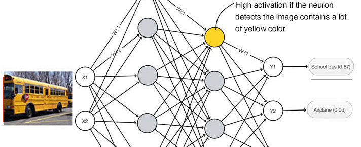
如果我们将毕加索的肖像画“Portrait of woman in d`hermine pass”输入到一个CNN分类器,那么此分类器有多大几率将其识别 为一个真正的人脸? 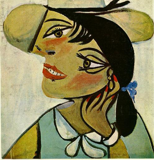
CNN擅长检测特征,但对于特征(透视、大小、方向)之间的空间关系检测效果较差。例如,下面的图片可能会欺骗一个简单的 CNN模型,使其认为这是一个很好的素描的人的脸。 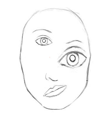
一个简单的CNN模型可以正确地提取鼻子、眼睛和嘴巴的特征,但在进行面部检测时会错误地激活神经元。由于没有实现空间方向和大小的匹配,人脸检测的激活值会变得过高。 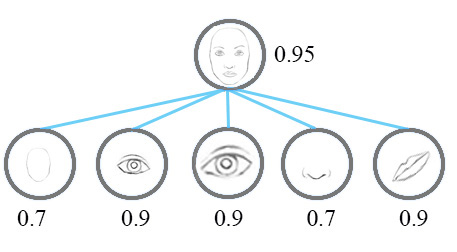
现在,我们假设每个神经元包含特征的可能性和属性。例如,它输出一个包含(可能性,方向,大小)的向量。利用这种空间信息,我们可以检测出鼻子、眼睛和耳朵等特征在方向和大小上的一致性,从而输出一个低得多的面部检测激活值。 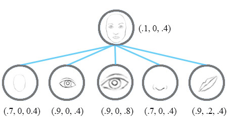 论文中并没有使用术语Neurons,而是使用了Capsules来表明胶囊输出一个向量,而不是一个单一的标量值。
同变性
论文中并没有使用术语Neurons,而是使用了Capsules来表明胶囊输出一个向量,而不是一个单一的标量值。
同变性
从概念上讲,CNN模型使用多个神经元和层来捕获不同的特征变量: 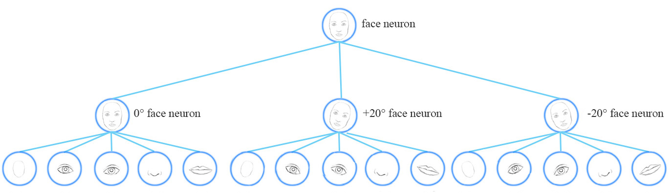
一个胶囊网络共享相同的胶囊来检测一个简单网络中的多个变体。 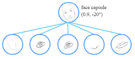
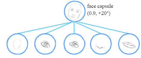
同变性是可以相互变换的对象的检测。直观地说,一个胶囊检测到脸右旋转20°(或左旋转20°),并不是通过匹配一个右旋转20°的变体来识别到脸部。通过迫使模型在胶囊中学习特征变量,我们可以用较少的训练数据更有效地推断可能的变体。 MNIST数据集包含55000个训练数据,即每位数5500个样本。然而,小孩子们不太可能阅读大量的样本来学习数字识别。我们现有的深度学习模型包括CNN在利用数据时显得效率低下。 With feature property as part of the information extracted by capsules, we may generalize the model better without an over extensive amount of labeled data. 胶囊(Capsule)A capsule is a group of neurons that not only capture the likelihood but also the parameters of the specific feature. 例如,下面的第一行表示由神经元检测到数字“7”的概率。一个二维胶囊由2个神经元组成。这个胶囊输出一个二维向量来检测数字“7”。对于第一张图像的第二排,它输出向量 v=(0,0.9) v = ( 0 , 0.9 ) 。向量的大小 ||v||=02+0.92−−−−−−−√=0.9 | | v | | = 0 2 + 0.9 2 = 0.9 对应检测到“7”的概率。每一行的第二个图像看起来更像是“1”而不是“7”。因此,其相应的可能性为“7”的概率更小(更小的标量值或向量大小但方向相同)。 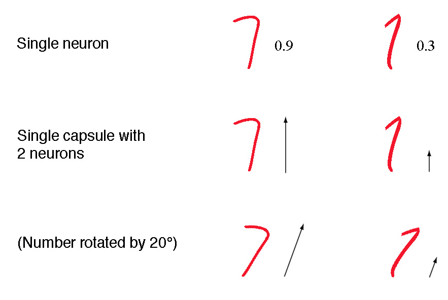
在第三行中,我们将图像旋转20°。该胶囊将产生相同大小但不同方向的向量。这里,向量的角度代表“7”的旋转角度。我们可以想象,完全可以在一个胶囊中再增加2个神经元来捕捉大小和宽度。 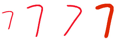
We call the output vector of a capsule as the activity vector with magnitude represents the probability of detecting a feature and its orientation represents its parameters (properties). 动态路由动态路由将胶囊分组形成父胶囊,并计算胶囊的输出。 直觉我们收集了3个不同大小和方向的相似草图,并以像素为单位测量了嘴巴和眼睛的水平宽度。其中 s(1)=(100,66),s(2)=(200,131),s(3)=(50,33). s ( 1 ) = ( 100 , 66 ) , s ( 2 ) = ( 200 , 131 ) , s ( 3 ) = ( 50 , 33 ) . 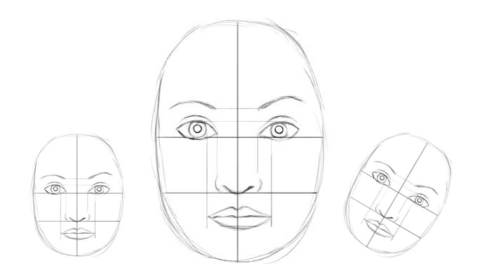 假设
Wm=2,We=3
W
m
=
2
,
W
e
=
3
,对于
s(1)
s
(
1
)
我们得到一个来自嘴巴和眼睛的投票:
假设
Wm=2,We=3
W
m
=
2
,
W
e
=
3
,对于
s(1)
s
(
1
)
我们得到一个来自嘴巴和眼睛的投票:
 我们看到
v(1)m
v
m
(
1
)
和
v(1)e
v
e
(
1
)
非常相似。当我们用其他的草图重复此操作时,得到了同样的发现。因此,嘴巴胶囊和眼睛胶囊可能与父胶囊紧密相关,宽度约为200像素。从经验来看,人脸是嘴巴的2倍宽(
Wm=2
W
m
=
2
),一只眼睛的3倍宽(
We=3
W
e
=
3
)。所以我们检测到的父胶囊是一个人脸胶囊。当然,我们可以通过添加更多的属性,如高度或颜色,使其更准确。在动态路由中,我们用一个变换矩阵
W
W
去转换输入胶囊的向量,构成一个投票,并用相似的投票分组。这些选票最终成为父胶囊的输出向量。那么我们怎么得到WW呢?只需在深度学习方法中进行:通过成本函数反向传播。
计算胶囊输出
我们看到
v(1)m
v
m
(
1
)
和
v(1)e
v
e
(
1
)
非常相似。当我们用其他的草图重复此操作时,得到了同样的发现。因此,嘴巴胶囊和眼睛胶囊可能与父胶囊紧密相关,宽度约为200像素。从经验来看,人脸是嘴巴的2倍宽(
Wm=2
W
m
=
2
),一只眼睛的3倍宽(
We=3
W
e
=
3
)。所以我们检测到的父胶囊是一个人脸胶囊。当然,我们可以通过添加更多的属性,如高度或颜色,使其更准确。在动态路由中,我们用一个变换矩阵
W
W
去转换输入胶囊的向量,构成一个投票,并用相似的投票分组。这些选票最终成为父胶囊的输出向量。那么我们怎么得到WW呢?只需在深度学习方法中进行:通过成本函数反向传播。
计算胶囊输出
对于一个胶囊来说,输入 ui u i 和输出 vj v j 都是向量。 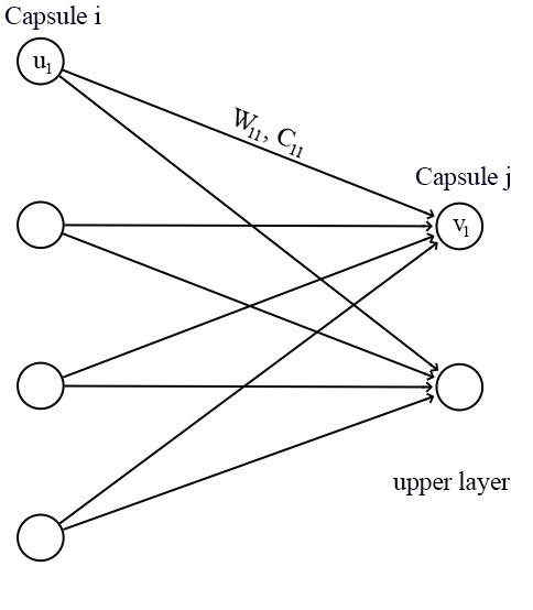
我们将变换矩阵
Wij
W
i
j
与前一层胶囊的输出
ui
u
i
相乘。例如,对于一个
p×k
p
×
k
矩阵,将
ui
u
i
转换为
u^j|i
u
^
j
|
i
,维度从k变为p,
((p×k)×(k×1)⟹p×1)
(
(
p
×
k
)
×
(
k
×
1
)
⟹
p
×
1
)
。然后根据权重
cij
c
i
j
计算加权和
sj
s
j
。 对于
sj
s
j
的激活函数,我们采用squashing而不是ReLU,所以胶囊的最终输出向量
vj
v
j
的长度在0到1之间。该函数将小向量压缩为零,大向量压缩为单位向量。 在胶囊中,我们通过迭代的动态路由计算中间值 cij c i j (耦合系数)来计算胶囊的输出。 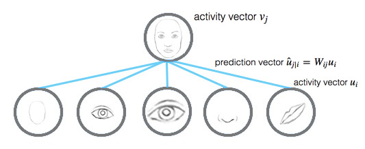 由上节可知,
预测向量
u^j|i
u
^
j
|
i
可以通过下式计算得到:
由上节可知,
预测向量
u^j|i
u
^
j
|
i
可以通过下式计算得到:
 而
激活向量
vj
v
j
(胶囊
j
j
的输出)为:
而
激活向量
vj
v
j
(胶囊
j
j
的输出)为:

直观上看,预测向量u^j|iu^j|i是来自胶囊
i
i
的预测(投票)并对胶囊jj的输出产生影响。如果激活向量与预测向量有很高的相似度,那么我们就可以断定这两个胶囊是高度相关的。这种相似性是通过预测向量和激活向量的标量积来度量的。
因此,相似度得分 bij b i j 会同时考虑到可能性和特征属性,而不像神经元只考虑可能性。同时,如果胶囊 i i 的激活uiui很低,由于 u^j|i u ^ j | i 的长度与 ui u i 成正比, bij b i j 仍然会较低,即如果嘴巴胶囊没有激活, bij b i j 在嘴巴胶囊和人脸胶囊之间仍然很低。 耦合系数
cij
c
i
j
由
bij
b
i
j
的softmax计算得到: 下面是动态路由的最终伪代码: 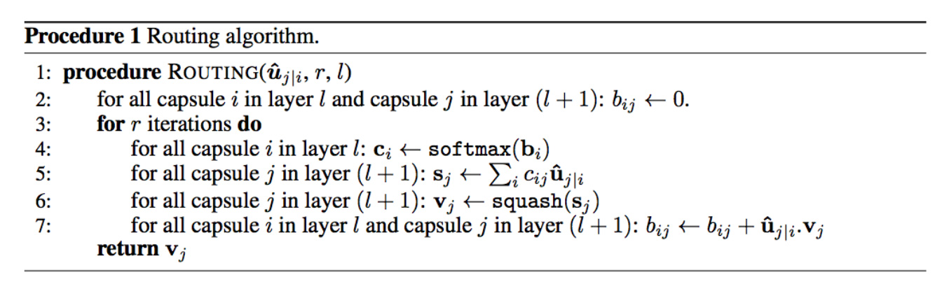
Routing a capsule to the capsule in the layer above based on relevancy is called Routing-by-agreement. 动态路由并不能完全替代反向传播。转换矩阵 W W 仍然使用成本函数通过反向传播训练。我们只是使用动态路由来计算胶囊的输出。通过计算cijcij来量化胶囊与其父胶囊之间的连接。这个值很重要,但生命周期很短暂。对于每一个数据点,在进行动态路由计算之前,我们都将它重新初始化为0。在计算胶囊输出时,无论是训练或测试,都需要重新做动态路由计算。 最大池化的缺陷CNN中的最大池化处理了平移变化。如果一个特征稍微移动一下,只要它仍然在池化窗口中,就依然可以被检测到。然而,这种方法只保留最大的特征(最主要的)并且丢弃其他的特征,而胶囊则保留前一层的特征加权总和。因此,它更适合于检测重叠特征。例如,在手写字体中检测多个重叠的数字:  胶囊协议路由(routing-by-agreement)的意义
在一个全连接的神经网络中,我们通过下式计算神经元 W W 则通过全局成本函数使用反向传播算法来训练得到。而迭代动态路由提供了一种通过使用本地特征的属性来计算胶囊如何激活的替代方法。从理论上讲,这样可以更好更简单地组合胶囊,形成一个有更低的对抗风险的解析树。 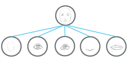
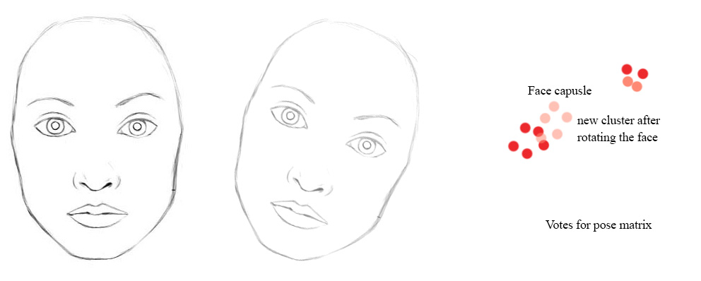
胶囊的迭代动态路由只是协议路由(routing-by-agreement)的一个展示。在关于胶囊的第二篇论文“Matrix capsules with EM routing”中,提出了一种新的基于期望最大化(EM)路由的矩阵胶囊[可能性,4x4姿态矩阵]。其姿态矩阵用来捕捉不同的视角,因此胶囊可以捕捉不同方位角和俯仰角的物体。 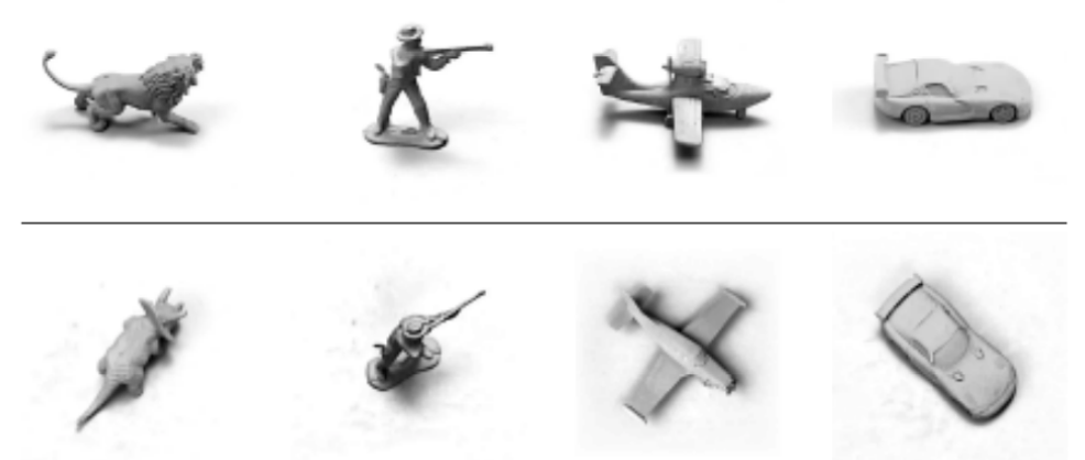 矩阵胶囊应用了一种聚类技术,EM路由(EM routing),将相关的胶囊聚集起来形成父胶囊。即使视角改变,投票也会通过一种协调的方式从下图中的红点变化到粉点。因此,EM路由仍然可以将相同的子胶囊聚集在一起。
 第一篇论文为深度学习打开了一个新的途径,第二篇论文则深入探讨了它的潜力。对于感兴趣的读者,我在第二篇关于矩阵胶囊的文章中有更多的细节。
胶囊网络的架构
第一篇论文为深度学习打开了一个新的途径,第二篇论文则深入探讨了它的潜力。对于感兴趣的读者,我在第二篇关于矩阵胶囊的文章中有更多的细节。
胶囊网络的架构
最后,我们应用胶囊构建胶囊网络进行MNIST数字分类。下面是一个使用了胶囊网络的架构。 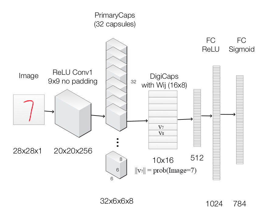
图像将喂给一个标准的卷积层ReLU Conv1。它使用256个9x9内核,产生256个通道的输出(特征映射)。其步长为1,无填充,将空间维数降低到20X20(28-9+1=20)。 然后数据进入一个修改过的用于支持胶囊的卷积层PrimaryCapsules。它生成一个8维向量而不是标量。PrimaryCapsules通过8x32个卷积核生成32个8维的胶囊(即8个输出神经元组合在一起构成一个胶囊)。PrimaryCapsules采用9x9卷积核,步长为2,无填充,将空间维度从20x20减小到到6x6(⌊20−92⌋+1=6⌊20−92⌋+1=6)。在PrimaryCapsules中,共有32x6x6个胶囊。 然后数据进入DigiCaps层,它通过一个形状为16x8的转换矩阵
Wij
W
i
j
将8维胶囊转换为16维胶囊,每一个胶囊对应于一个数字类别
j
j
(从1到10)。
因为有10个类别,DigiCaps的形状是10x16(10个16-D向量)。每个向量 vj v j 作为类别 j j 的胶囊。图像被分类为jj的概率可通过计算 ||vj|| | | v j | | 得到。在我们的例子中,图像的标签是7,而 v7 v 7 是我们输入的潜在表示。通过2个全连接隐藏层,我们可以从 v7 v 7 中重构 28x28的图像。 下面是每一层的摘要: 层使用输出形状Image原图像阵列28x28x1ReLU Conv1卷积层,9x9内核,256个通道,步长1,无填充,ReLU激活20x20x256PrimaryCapsules卷积胶囊层,9x9内核,输出32x6x6个8维胶囊,步长2,无填充6x6x32x8DigiCaps胶囊的输出由 Wij W i j 计算得到( i i 从1到32x6x6,jj从1到10)10x16FC1全连接层,ReLU激活512FC2全连接层,ReLU激活1024Output image全连接层,sigmoid激活784 (28x28)Our capsule layers use convolution kernels to explore locality information. 损失函数(Margin loss)在我们的示例中,我们希望检测一张图片中的多个数字。胶囊对于出现在画面中的每个类别的数字
c
c
使用一个单独的边距损失LcLc: 如果一个类别的对象存在时 Tc=1 T c = 1 。 m+=0.9,m−=−0.1 m + = 0.9 , m − = − 0.1 。 λ λ 下加权(默认为0.5)通过收缩所有类的激活向量停止初始学习。总损失即是所有类别的损失的总和。 在Keras中计算边距: def margin_loss(y_true, y_pred): """ :param y_true: [None, n_classes] :param y_pred: [None, num_capsule] :return: a scalar loss value. """ L = y_true * K.square(K.maximum(0., 0.9 - y_pred)) + \ 0.5 * (1 - y_true) * K.square(K.maximum(0., y_pred - 0.1)) return K.mean(K.sum(L, 1)) 胶囊网络模型这里是一个由Keras实现的构建胶囊网络模型的代码: def CapsNet(input_shape, n_class, num_routing): """ :param input_shape: (None, width, height, channels) :param n_class: number of classes :param num_routing: number of routing iterations :return: A Keras Model with 2 inputs (image, label) and 2 outputs (capsule output and reconstruct image) """ # Image x = layers.Input(shape=input_shape) # ReLU Conv1 conv1 = layers.Conv2D(filters=256, kernel_size=9, strides=1, padding='valid', activation='relu', name='conv1')(x) # PrimaryCapsules: Conv2D layer with `squash` activation, # reshape to [None, num_capsule, dim_vector] primarycaps = PrimaryCap(conv1, dim_vector=8, n_channels=32, kernel_size=9, strides=2, padding='valid') # DigiCap: Capsule layer. Routing algorithm works here. digitcaps = DigiCaps(num_capsule=n_class, dim_vector=16, num_routing=num_routing, name='digitcaps')(primarycaps) # The length of the capsule's output vector out_caps = Length(name='out_caps')(digitcaps) # Decoder network. y = layers.Input(shape=(n_class,)) # The true label is used to extract the corresponding vj masked = Mask()([digitcaps, y]) x_recon = layers.Dense(512, activation='relu')(masked) x_recon = layers.Dense(1024, activation='relu')(x_recon) x_recon = layers.Dense(784, activation='sigmoid')(x_recon) x_recon = layers.Reshape(target_shape=[28, 28, 1], name='out_recon')(x_recon) # two-input-two-output keras Model return models.Model([x, y], [out_caps, x_recon])该胶囊的输出向量 ||vj|| | | v j | | 的长度对应于它属于类别 j j 的概率。例如,||v7||||v7||是输入图像为7的概率。 class Length(layers.Layer): def call(self, inputs, **kwargs): # L2 length which is the square root # of the sum of square of the capsule element return K.sqrt(K.sum(K.square(inputs), -1)) PrimaryCapsulesPrimaryCapsules将20x20 256通道数据转换为32x6x6的8维胶囊。 def PrimaryCap(inputs, dim_vector, n_channels, kernel_size, strides, padding): """ Apply Conv2D `n_channels` times and concatenate all capsules :param inputs: 4D tensor, shape=[None, width, height, channels] :param dim_vector: the dim of the output vector of capsule :param n_channels: the number of types of capsules :return: output tensor, shape=[None, num_capsule, dim_vector] """ output = layers.Conv2D(filters=dim_vector*n_channels, kernel_size=kernel_size, strides=strides, padding=padding)(inputs) outputs = layers.Reshape(target_shape=[-1, dim_vector])(output) return layers.Lambda(squash)(outputs) Squash functionSquash函数的行为类似于sigmoid,它将向量压缩,使其长度在0到1之间。 DigiCaps将PrimaryCapsules层中的胶囊转换为10个胶囊,每个代表一个类别 j j 的预测。以下是构造10个类别16维胶囊的代码: # num_routing is default to 3 digitcaps = DigiCap(num_capsule=n_class, dim_vector=16, num_routing=num_routing, name='digitcaps')(primarycaps)DigiCaps只是一个简单的全连接层的扩展。它取一个向量并输出一个向量,而不是取标量并输出标量: input shape = (None, input_num_capsule (32), input_dim_vector(8) )output shape = (None, num_capsule (10), dim_vector(16) ) 这里是DigiCaps的代码,我们稍后将详细解释代码的某些部分。 class DigiCap(layers.Layer): """ The capsule layer. :param num_capsule: number of capsules in this layer :param dim_vector: dimension of the output vectors of the capsules in this layer :param num_routings: number of iterations for the routing algorithm """ def __init__(self, num_capsule, dim_vector, num_routing=3, kernel_initializer='glorot_uniform', b_initializer='zeros', **kwargs): super(DigiCap, self).__init__(**kwargs) self.num_capsule = num_capsule # 10 self.dim_vector = dim_vector # 16 self.num_routing = num_routing # 3 self.kernel_initializer = initializers.get(kernel_initializer) self.b_initializer = initializers.get(b_initializer) def build(self, input_shape): "The input Tensor should have shape=[None, input_num_capsule, input_dim_vector]" assert len(input_shape) >= 3, self.input_num_capsule = input_shape[1] self.input_dim_vector = input_shape[2] # Transform matrix W self.W = self.add_weight(shape=[self.input_num_capsule, self.num_capsule, self.input_dim_vector, self.dim_vector], initializer=self.kernel_initializer, name='W') # Coupling coefficient. # The redundant dimensions are just to facilitate subsequent matrix calculation. self.b = self.add_weight(shape=[1, self.input_num_capsule, self.num_capsule, 1, 1], initializer=self.b_initializer, name='b', trainable=False) self.built = True def call(self, inputs, training=None): # inputs.shape = (None, input_num_capsule, input_dim_vector) # Expand dims to (None, input_num_capsule, 1, 1, input_dim_vector) inputs_expand = K.expand_dims(K.expand_dims(inputs, 2), 2) # Replicate num_capsule dimension to prepare being multiplied by W # Now shape = [None, input_num_capsule, num_capsule, 1, input_dim_vector] inputs_tiled = K.tile(inputs_expand, [1, 1, self.num_capsule, 1, 1]) # Compute `inputs * W` by scanning inputs_tiled on dimension 0. # inputs_hat.shape = [None, input_num_capsule, num_capsule, 1, dim_vector] inputs_hat = tf.scan(lambda ac, x: K.batch_dot(x, self.W, [3, 2]), elems=inputs_tiled, initializer=K.zeros([self.input_num_capsule, self.num_capsule, 1, self.dim_vector])) # Routing algorithm assert self.num_routing > 0, 'The num_routing should be > 0.' for i in range(self.num_routing): c = tf.nn.softmax(self.b, dim=2) # dim=2 is the num_capsule dimension # outputs.shape=[None, 1, num_capsule, 1, dim_vector] outputs = squash(K.sum(c * inputs_hat, 1, keepdims=True)) # last iteration needs not compute b which will not be passed to the graph any more anyway. if i != self.num_routing - 1: self.b += K.sum(inputs_hat * outputs, -1, keepdims=True) return K.reshape(outputs, [-1, self.num_capsule, self.dim_vector])build方法声明了self.W参数和self.b参数,分别代表转换矩阵WW和 bij b i j def build(self, input_shape): "The input Tensor should have shape=[None, input_num_capsule, input_dim_vector]" assert len(input_shape) >= 3, self.input_num_capsule = input_shape[1] self.input_dim_vector = input_shape[2] # Transform matrix W self.W = self.add_weight(shape=[self.input_num_capsule, self.num_capsule, self.input_dim_vector, self.dim_vector], initializer=self.kernel_initializer, name='W') # Coupling coefficient. # The redundant dimensions are just to facilitate subsequent matrix calculation. self.b = self.add_weight(shape=[1, self.input_num_capsule, self.num_capsule, 1, 1], initializer=self.b_initializer, name='b', trainable=False) self.built = True为了计算: 代码首先展开了 ui u i 的维度,然后与 w w 相乘。然而,考虑到运行速度,对WijuiWijui的简单点积的实现(见注释)由tf.scan取代。 class DigiCap(layers.Layer): ... def call(self, inputs, training=None): # inputs.shape = (None, input_num_capsule, input_dim_vector) # Expand dims to (None, input_num_capsule, 1, 1, input_dim_vector) inputs_expand = K.expand_dims(K.expand_dims(inputs, 2), 2) # Replicate num_capsule dimension to prepare being multiplied by W # Now shape = [None, input_num_capsule, num_capsule, 1, input_dim_vector] inputs_tiled = K.tile(inputs_expand, [1, 1, self.num_capsule, 1, 1]) """ # Compute `inputs * W` # By expanding the first dim of W. # W has shape (batch_size, input_num_capsule, num_capsule, input_dim_vector, dim_vector) w_tiled = K.tile(K.expand_dims(self.W, 0), [self.batch_size, 1, 1, 1, 1]) # Transformed vectors, inputs_hat.shape = (None, input_num_capsule, num_capsule, 1, dim_vector) inputs_hat = K.batch_dot(inputs_tiled, w_tiled, [4, 3]) """ # However, we will implement the same code with a faster implementation using tf.sacn # Compute `inputs * W` by scanning inputs_tiled on dimension 0. # inputs_hat.shape = [None, input_num_capsule, num_capsule, 1, dim_vector] inputs_hat = tf.scan(lambda ac, x: K.batch_dot(x, self.W, [3, 2]), elems=inputs_tiled, initializer=K.zeros([self.input_num_capsule, self.num_capsule, 1, self.dim_vector]))下面是迭代动态路由的伪代码实现。
class DigiCap(layers.Layer):
...
def call(self, inputs, training=None):
...
# Routing algorithm
assert self.num_routing > 0, 'The num_routing should be > 0.'
for i in range(self.num_routing): # Default: loop 3 times
c = tf.nn.softmax(self.b, dim=2) # dim=2 is the num_capsule dimension
# outputs.shape=[None, 1, num_capsule, 1, dim_vector]
outputs = squash(K.sum(c * inputs_hat, 1, keepdims=True))
# last iteration needs not compute b which will not be passed to the graph any more anyway.
if i != self.num_routing - 1:
self.b += K.sum(inputs_hat * outputs, -1, keepdims=True)
return K.reshape(outputs, [-1, self.num_capsule, self.dim_vector])
图像重构
在训练中我们用真实的标签来选择 vj v j 并重建图像。然后我们通过将 vj v j 喂到 3个全连接层来重新生成原始图像。 在训练中用mask方法选择 vj v j class Mask(layers.Layer): """ Mask a Tensor with shape=[None, d1, d2] by the max value in axis=1. Output shape: [None, d2] """ def call(self, inputs, **kwargs): # use true label to select target capsule, shape=[batch_size, num_capsule] if type(inputs) is list: # true label is provided with shape = [batch_size, n_classes], i.e. one-hot code. assert len(inputs) == 2 inputs, mask = inputs else: # if no true label, mask by the max length of vectors of capsules x = inputs # Enlarge the range of values in x to make max(new_x)=1 and others < 0 x = (x - K.max(x, 1, True)) / K.epsilon() + 1 mask = K.clip(x, 0, 1) # the max value in x clipped to 1 and other to 0 # masked inputs, shape = [batch_size, dim_vector] inputs_masked = K.batch_dot(inputs, mask, [1, 1]) return inputs_masked 重构损失将重构的损失 ||image−reconstructedimage|| | | i m a g e − r e c o n s t r u c t e d i m a g e | | 加入损失函数。训练网络并捕捉关键属性到胶囊中。然而,重构损失将会与一个正则因子(0.0005)相乘,所以它不主导边际损失。 胶囊到底学到了什么?在DigiCaps中的每个胶囊都是一个16-D的向量。稍微改变其中一个维度而保持其他维为常数,我们会看到每个维度捕获到了什么样的属性。下面的每一行都是只改变了一维的重构图像(使用解码器)。 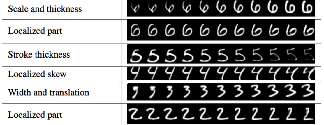 Sabour的实现
Sara Sabour在GitHub发布了一个胶囊实现 Github Sara Sabour。由于这是一个正在进行的研究,期望实现可能与论文有所不同。 原文链接:https://jhui.github.io/2017/11/03/Dynamic-Routing-Between-Capsules/ |
 cij
c
i
j
为耦合系数,通过迭代的动态路由(将在下面讨论)过程计算得到,并且规定
∑jcij
∑
j
c
i
j
和为1,从概念上讲,
cij
c
i
j
衡量胶囊
i
i
有多大可能激活胶囊jj。
cij
c
i
j
为耦合系数,通过迭代的动态路由(将在下面讨论)过程计算得到,并且规定
∑jcij
∑
j
c
i
j
和为1,从概念上讲,
cij
c
i
j
衡量胶囊
i
i
有多大可能激活胶囊jj。


 类别jj最终的输出
vj
v
j
为:
类别jj最终的输出
vj
v
j
为: 


【本文地址】