设函数 y = f ( x ) {\displaystyle y=f(x)\,\!} 在点 x 0 {\displaystyle \;x_{0}\;} 的某个邻域内有定义，当自变量 x {\displaystyle \;x\;} 在 x 0 {\displaystyle \;x_{0}\;} 处取得增量 Δ x {\displaystyle \Delta x} （点 x 0 + Δ x {\displaystyle \;x_{0}+\Delta x} 仍在该邻域内）时，相应地函数 y {\displaystyle \;y\;} 取得增量 Δ y = f ( x 0 + Δ x ) − f ( x 0 ) {\displaystyle \Delta y=f(x_{0}+\Delta x)-f(x_{0})\,\!} ；如果 Δ {\displaystyle \Delta } y {\displaystyle \;y\;} 与 Δ {\displaystyle \Delta } x {\displaystyle \;x\;} 之比当 Δ {\displaystyle \Delta } x → 0 {\displaystyle x\to 0} 时的极限存在，则称函数 y = f ( x ) {\displaystyle y=f(x)\,\!} 在点 x 0 {\displaystyle \;x_{0}\;} 处可导，并称这个极限为函数 y = f ( x ) {\displaystyle y=f(x)\,\!} 在点 x 0 {\displaystyle \;x_{0}\;} 处的导数，记为 f ′ ( x 0 ) {\displaystyle f'(x_{0})\;\!} ，即

f ′ ( x 0 ) = lim Δ x → 0 Δ y Δ x = lim Δ x → 0 f ( x 0 + Δ x ) − f ( x 0 ) Δ x {\displaystyle f'(x_{0})=\lim _{\Delta x\to 0}{\frac {\Delta y}{\Delta x}}=\lim _{\Delta x\to 0}{\frac {f(x_{0}+\Delta x)-f(x_{0})}{\Delta x}}} ，

也可记作 y ′ | x = x 0 {\displaystyle \left.y^{\prime }\right|_{x=x_{0}}} ， d y d x | x = x 0 {\displaystyle \left.{\frac {\mathrm {d} y}{\mathrm {d} x}}\right|_{x=x_{0}}} 或 d f ( x ) d x | x = x 0 {\displaystyle \left.{\frac {\mathrm {d} f(x)}{\mathrm {d} x}}\right|_{x=x_{0}}}

若将一点扩展成函数 f ( x ) {\displaystyle f(x)} 在其定义域包含的某开区间 I {\displaystyle I} 内每一个点，那么函数 f ( x ) {\displaystyle f(x)} 在开区间 I {\displaystyle \;I\;} 内可导，这时对于 I {\displaystyle \;I\;} 内每一个确定的 x {\displaystyle \;x\;} 值，都对应着 f ( x ) {\displaystyle f(x)} 的一个确定的导数，如此一来每一个导数就构成了一个新的函数，这个函数称作原函数 f ( x ) {\displaystyle f(x)} 的导函数，记作： y ′ {\displaystyle y'} 、 f ′ ( x ) {\displaystyle f'(x)\;\!} 或者 d f ( x ) d x {\displaystyle {\frac {\mathrm {d} f(x)}{\mathrm {d} x}}}

导函数的定义表达式为：

f ′ ( x ) = lim Δ x → 0 f ( x + Δ x ) − f ( x ) Δ x {\displaystyle f'(x)=\lim _{\Delta x\to 0}{\frac {f(x+\Delta x)-f(x)}{\Delta x}}}

值得注意的是，导数是一个数，是指函数 f ( x ) {\displaystyle f(x)} 在点 x 0 {\displaystyle x_{0}} 处导函数的函数值。但通常也可以说导函数为导数，其区别仅在于一个点还是连续的点。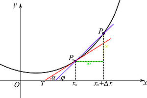

如右图所示，设 P 0 {\displaystyle P_{0}} 为曲线上的一个定点， P {\displaystyle P} 为曲线上的一个动点。当 P {\displaystyle P} 沿曲线逐渐趋向于点 P 0 {\displaystyle P_{0}} 时，并且割线 P P 0 {\displaystyle PP_{0}} 的极限位置 P 0 T {\displaystyle P_{0}T} 存在，则称 P 0 T {\displaystyle P_{0}T} 为曲线在 P 0 {\displaystyle P_{0}} 处的切线。

若曲线为一函数 y = f ( x ) {\displaystyle y=f(x)} 的图像，那么割线 P P 0 {\displaystyle PP_{0}} 的斜率为：

tan ⁡ φ = Δ y Δ x = f ( x 0 + Δ x ) − f ( x 0 ) Δ x {\displaystyle \tan \varphi ={\frac {\Delta y}{\Delta x}}={\frac {f(x_{0}+\Delta x)-f(x_{0})}{\Delta x}}}

当 P 0 {\displaystyle P_{0}} 处的切线 P 0 T {\displaystyle P_{0}T} ，即 P P 0 {\displaystyle PP_{0}} 的极限位置存在时，此时 Δ x → 0 {\displaystyle \Delta x\to 0} ， φ → α {\displaystyle \varphi \to \alpha } ，则 P 0 T {\displaystyle P_{0}T} 的斜率 tan ⁡ α {\displaystyle \tan \alpha } 为：

tan ⁡ α = lim Δ x → 0 tan ⁡ φ = lim Δ x → 0 f ( x 0 + Δ x ) − f ( x 0 ) Δ x {\displaystyle \tan \alpha =\lim _{\Delta x\to 0}\tan \varphi =\lim _{\Delta x\to 0}{\frac {f(x_{0}+\Delta x)-f(x_{0})}{\Delta x}}}

上式与一般定义中的导数定义是完全相同，则 f ′ ( x 0 ) = tan ⁡ α {\displaystyle f'(x_{0})=\tan \alpha } ，故导数的几何意义即曲线 y = f ( x ) {\displaystyle y=f(x)} 在点 P 0 ( x 0 , f ( x 0 ) ) {\displaystyle P_{0}(x_{0},f(x_{0}))} 处切线的斜率。

如果一个函数的定义域为全体实数，即函数在 ( − ∞ , + ∞ ) {\displaystyle (-\infty ,+\infty )} 上都有定义，那么该函数是不是在定义域上处处可导呢？答案是否定的。函数在定义域中一点可导需要一定的条件是：函数在该点的左右两侧导数都存在且相等。这实际上是按照极限存在的一个充要条件（极限存在，它的左右极限存在且相等）推导而来：

lim Δ x → 0 f ( x 0 + Δ x ) − f ( x 0 ) Δ x = lim Δ x → 0 − f ( x 0 + Δ x ) − f ( x 0 ) Δ x = lim Δ x → 0 + f ( x 0 + Δ x ) − f ( x 0 ) Δ x {\displaystyle \lim _{\Delta x\to 0}{\frac {f(x_{0}+\Delta x)-f(x_{0})}{\Delta x}}=\lim _{\Delta x\to 0^{-}}{\frac {f(x_{0}+\Delta x)-f(x_{0})}{\Delta x}}=\lim _{\Delta x\to 0^{+}}{\frac {f(x_{0}+\Delta x)-f(x_{0})}{\Delta x}}}

上式中，后两个式子可以定义为函数在 x 0 {\displaystyle x_{0}} 处的左右导数：

用两个函数的例子来说明函数可导的条件。

1.上面这个符号函数在 x = 0 {\displaystyle x=0} 处可导吗？

2.上面这个绝对值函数在 x = 0 {\displaystyle x=0} 处可导吗？

以上两个函数都是在定义域内连续的函数，由此就可以得出一个结论：连续的函数不一定处处可导。

但处处可导的函数一定处处连续。

Δ y = f ( x 0 + Δ x ) − f ( x 0 ) {\displaystyle \Delta y=f(x_{0}+\Delta x)-f(x_{0})}

所以： lim Δ x → 0 Δ y = lim Δ x → 0 ( Δ y Δ x ⋅ Δ x ) = lim Δ x → 0 Δ y Δ x ⋅ lim Δ x → 0 Δ x = 0 {\displaystyle \lim _{\Delta x\to 0}\Delta y=\lim _{\Delta x\to 0}\left({\frac {\Delta y}{\Delta x}}\cdot \Delta x\right)=\lim _{\Delta x\to 0}{\frac {\Delta y}{\Delta x}}\cdot \lim _{\Delta x\to 0}\Delta x=0}

在解决函数的导数问题上，利用定义是在过于麻烦。故利用定义来引申出几个基本的求导法则，以利于更好地解决各类求导的问题。

特别地，对于常数 C {\displaystyle C} ：

以上法则的证明中，对于1，可以利用极限的运算法则验证；对于2，可以直接使用导数定义证明，证明如下：

或

我们可以用一个例子来说明：试求函数 y = arcsin ⁡ x ( | x | 0}">因此由反函数求导法则可得：在对应区间 I y = ( − 1 , 1 ) {\displaystyle I_{y}=(-1,1)} 内有：

( arcsin ⁡ x ) ′ = 1 ( sin ⁡ y ) ′ = 1 cos ⁡ y = 1 1 − sin 2 ⁡ y = 1 1 − x 2 {\displaystyle (\arcsin x)'={\frac {1}{(\sin y)'}}={\frac {1}{\cos y}}={\frac {1}{\sqrt {1-\sin ^{2}y}}}={\frac {1}{\sqrt {1-x^{2}}}}}

对于参数方程： { x = ψ ( t ) y = ϕ ( t ) ( α ≤ t ≤ β ) {\displaystyle {\begin{cases}x=\psi (t)\\y=\phi (t)\end{cases}}(\alpha \leq t\leq \beta )} ,其中 ϕ ( t ) {\displaystyle \phi (t)} 和 ψ ( t ) {\displaystyle \psi (t)} 可导，且 x = ψ ( t ) {\displaystyle x=\psi (t)} 严格单调(?)， ψ ′ ( t ) ≠ 0 {\displaystyle \psi '(t)\neq 0} ，根据复合函数求导法则和反函数求导法则可得参数方程的导数为：

d y d x = d y d t ⋅ d t d x = d y d t ⋅ 1 d x d t = ϕ ′ ( t ) ψ ′ ( t ) {\displaystyle {\frac {dy}{dx}}={\frac {dy}{dt}}\cdot {\frac {dt}{dx}}={\frac {dy}{dt}}\cdot {\frac {1}{\frac {dx}{dt}}}={\frac {\phi '(t)}{\psi '(t)}}}

对于极坐标方程 { x = ρ ( θ ) cos ⁡ θ y = ρ ( θ ) sin ⁡ θ {\displaystyle {\begin{cases}x=\rho (\theta )\cos \theta \\y=\rho (\theta )\sin \theta \end{cases}}} ，根据参数方程的求导法则可得极坐标方程的导数为：

d y d x = [ ρ ( θ ) sin ⁡ θ ] ′ [ ρ ( θ ) cos ⁡ θ ] ′ = ρ θ ′ sin ⁡ θ + ρ cos ⁡ θ ρ θ ′ cos ⁡ θ − ρ sin ⁡ θ {\displaystyle {\frac {dy}{dx}}={\frac {\left[\rho (\theta )\sin \theta \right]'}{\left[\rho (\theta )\cos \theta \right]'}}={\frac {\rho _{\theta }^{'}\sin \theta +\rho \cos \theta }{\rho _{\theta }^{'}\cos \theta -\rho \sin \theta }}}

隐函数的求导方法的基本思想是要把方程 F ( x , y ) = 0 {\displaystyle F(x,y)=0} 中的看作 x {\displaystyle x} 的函数 y ( x ) {\displaystyle y(x)} ，方程两端对 x {\displaystyle x} 求导，然后再解出隐函数的导数 d y d x {\displaystyle {\frac {dy}{dx}}} 。

d ( x 1 2 + y 1 2 ) d x = d a d x {\displaystyle {\frac {d(x^{\frac {1}{2}}+y^{\frac {1}{2}})}{dx}}={\frac {d{\sqrt {a}}}{dx}}}

1 2 x − 1 2 + 1 2 y − 1 2 ⋅ d y d x = 0 {\displaystyle {\frac {1}{2}}x^{-{\frac {1}{2}}}+{\frac {1}{2}}y^{-{\frac {1}{2}}}\cdot {\frac {dy}{dx}}=0}

d y d x = − y x ( x , y > 0 ) {\displaystyle {\frac {dy}{dx}}=-{\sqrt {\frac {y}{x}}}(x,y>0)}

参数方程的高阶求导

对于参数方程： { x = ψ ( t ) y = ϕ ( t ) {\displaystyle {\begin{cases}x=\psi (t)\\y=\phi (t)\end{cases}}} ，其中 ϕ ( t ) {\displaystyle \phi (t)} 和 ψ ( t ) {\displaystyle \psi (t)} 二阶可导，且 ψ ′ ( t ) ≠ 0 {\displaystyle \psi '(t)\neq 0} ，则由 d y d x = ϕ ′ ( t ) ψ ′ ( t ) {\displaystyle {\frac {dy}{dx}}={\frac {\phi '(t)}{\psi '(t)}}} ，有

d 2 y d x 2 {\displaystyle {\frac {{{\rm {d}}^{2}}y}{{\rm {d}}{x^{2}}}}} = d d x ( d y d x ) {\displaystyle ={\frac {\rm {d}}{{\rm {d}}x}}\left({\frac {{\rm {d}}y}{{\rm {d}}x}}\right)}

= d d x ( ϕ ′ ( t ) ψ ′ ( t ) ) {\displaystyle ={\frac {\rm {d}}{{\rm {d}}x}}\left({\frac {\phi '(t)}{\psi '(t)}}\right)}

= d d t ( ϕ ′ ( t ) ψ ′ ( t ) ) ⋅ d t d x {\displaystyle ={\frac {\rm {d}}{{\rm {d}}t}}\left({\frac {\phi '(t)}{\psi '(t)}}\right)\cdot {\frac {{\rm {d}}t}{{\rm {d}}x}}}

= ϕ ″ ( t ) ψ ′ ( t ) − ϕ ′ ( t ) ψ ″ ( t ) [ ψ ′ ( t ) ] 2 ⋅ 1 ψ ′ ( t ) {\displaystyle ={\frac {\phi ''(t)\psi '(t)-\phi '(t)\psi ''(t)}{{[\psi '(t)]}^{2}}}\cdot {\frac {1}{\psi '(t)}}}

物理学、几何学、经济学等学科中的一些重要概念都可以用导数来表示。例如，在物理学中，速度被定义为位置函数的导数，即： v ( t ) = d s d t {\displaystyle v(t)={ds \over dt}} ；而加速度被定义为速度函数的导数，即： a ( t ) = d v d t {\displaystyle a(t)={dv \over dt}} 。另外，导数还可以表示曲线在一点的斜率，以及经济学中的边际和弹性。