深度学习笔记(二十)网络的参数量(param) 和浮点计算量(FLOPs) |
您所在的位置:网站首页 › 神经网络计算量统计 › 深度学习笔记(二十)网络的参数量(param) 和浮点计算量(FLOPs) |
深度学习笔记(二十)网络的参数量(param) 和浮点计算量(FLOPs)
|
参考: 1. CNN 模型所需的计算力(flops)和参数(parameters)数量是怎么计算的? 2. TensorFlow 模型浮点数计算量和参数量统计 3. How fast is my model? 计算公式理论上的计算公式如下: \begin{equation}\label{FLOPs}\begin{split}& param_{conv} = (k_w * k_h * c_{in}) * c_{out} + c_{out} \\& macc_{conv} = (k_w * k_h * c_{in}) * c_{out} * H * W \\& FLOPs_{conv} = [2 * (k_w * k_h * c_{in}) * c_{out} + c_{out}] * H * W \\& param_{fc} = (n_{in} * n_{out}) + n_{out} \\& macc_{fc} = n_{in} * n_{out} \\& FLOPs_{fc} = 2 * (n_{in} * n_{out}) + n_{out} \\\end{split}\end{equation} 注:以上公式是考虑常规卷积/全连接层操作且有 bias 的情况! 卷积层的参数量和卷积核的大小、输入输出通道数相关;全连接层的参数量则只与输入输出通道数有关。 MACCs:是multiply-accumulate operations,指点积运算, 一个 macc = 2FLOPs FLOPs 的全称是 floating points of operations,即浮点运算次数,用来衡量模型的计算复杂度。计算 FLOPs 实际上是计算模型中乘法和加法的运算次数。卷积层的浮点运算次数不仅取决于卷积核的大小和输入输出通道数,还取决于特征图的大小;而全连接层的浮点运算次数和参数量是相同的。 特别的,对于 Group Conv: \begin{equation}\label{GC_FLOPs}\begin{split}& param_{GC} = (k_w * k_h * \frac{c_{in}}{G}) * c_{out} + c_{out} \\& macc_{GC} = (k_w * k_h * \frac{c_{in}}{G}) * c_{out} * H * W \\& FLOPs_{GC} = [2 * (k_w * k_h * \frac{c_{in}}{G}) * c_{out} + c_{out}] * H * W \\\end{split}\end{equation} 手动计算简单起见,这里以 LeNet 为例:
我们这里先手工计算下: \begin{equation}\label{Example}\begin{split}& param_{conv1} = (5^2 * 1) * 20 + 20 = 520 \\& macc_{conv1} = (5^2 * 1) * 20 * 24 * 24 = 288k \\& FLOPs_{conv1} = 2 * macc_{conv1} + 20 * 24 * 24 = 587.52k \\& \\& FLOPs_{pool1} = 20 * 24 * 24 = 11.52k \\& \\& param_{conv2} = (5^2 * 20) * 50) + 50 = 25.05k \\& macc_{conv1} = (5^2 * 20) * 50 * 8 * 8 = 1.6M \\& FLOPs_{conv2} = 2 * macc_{conv2} + 50 * 8 * 8 = 3203.2k \\& \\& FLOPs_{pool2} = 50 * 8 * 8 = 3.2k \\& \\& param_{ip1} = (50*4*4) * 500 + 500 = 400.5k \\& macc_{ip1} = (50*4*4) * 500 = 400k \\& FLOPs_{ip1} = 2* macc_{ip1} + 500 = 800.5k \\&\\& param_{ip2} = 500 * 10 + 10 = 5.01k \\& macc_{ip2} = 500 * 10 = 5k \\& FLOPs_{ip2} = 2 * macc_{ip2} + 10 = 10.01k \\\end{split}\end{equation} Caffe  name: "LeNet"
input: "data"
input_shape {
dim: 1
dim: 1
dim: 28
dim: 28
}
layer {
name: "conv1"
type: "Convolution"
bottom: "data"
top: "conv1"
param {
lr_mult: 1
}
param {
lr_mult: 2
}
convolution_param {
num_output: 20
kernel_size: 5
stride: 1
weight_filler {
type: "xavier"
}
bias_filler {
type: "constant"
}
}
}
layer {
name: "pool1"
type: "Pooling"
bottom: "conv1"
top: "pool1"
pooling_param {
pool: MAX
kernel_size: 2
stride: 2
}
}
layer {
name: "conv2"
type: "Convolution"
bottom: "pool1"
top: "conv2"
param {
lr_mult: 1
}
param {
lr_mult: 2
}
convolution_param {
num_output: 50
kernel_size: 5
stride: 1
weight_filler {
type: "xavier"
}
bias_filler {
type: "constant"
}
}
}
layer {
name: "pool2"
type: "Pooling"
bottom: "conv2"
top: "pool2"
pooling_param {
pool: MAX
kernel_size: 2
stride: 2
}
}
layer {
name: "ip1"
type: "InnerProduct"
bottom: "pool2"
top: "ip1"
param {
lr_mult: 1
}
param {
lr_mult: 2
}
inner_product_param {
num_output: 500
weight_filler {
type: "xavier"
}
bias_filler {
type: "constant"
}
}
}
layer {
name: "relu1"
type: "ReLU"
bottom: "ip1"
top: "ip1"
}
layer {
name: "ip2"
type: "InnerProduct"
bottom: "ip1"
top: "ip2"
param {
lr_mult: 1
}
param {
lr_mult: 2
}
inner_product_param {
num_output: 10
weight_filler {
type: "xavier"
}
bias_filler {
type: "constant"
}
}
}
View Code
name: "LeNet"
input: "data"
input_shape {
dim: 1
dim: 1
dim: 28
dim: 28
}
layer {
name: "conv1"
type: "Convolution"
bottom: "data"
top: "conv1"
param {
lr_mult: 1
}
param {
lr_mult: 2
}
convolution_param {
num_output: 20
kernel_size: 5
stride: 1
weight_filler {
type: "xavier"
}
bias_filler {
type: "constant"
}
}
}
layer {
name: "pool1"
type: "Pooling"
bottom: "conv1"
top: "pool1"
pooling_param {
pool: MAX
kernel_size: 2
stride: 2
}
}
layer {
name: "conv2"
type: "Convolution"
bottom: "pool1"
top: "conv2"
param {
lr_mult: 1
}
param {
lr_mult: 2
}
convolution_param {
num_output: 50
kernel_size: 5
stride: 1
weight_filler {
type: "xavier"
}
bias_filler {
type: "constant"
}
}
}
layer {
name: "pool2"
type: "Pooling"
bottom: "conv2"
top: "pool2"
pooling_param {
pool: MAX
kernel_size: 2
stride: 2
}
}
layer {
name: "ip1"
type: "InnerProduct"
bottom: "pool2"
top: "ip1"
param {
lr_mult: 1
}
param {
lr_mult: 2
}
inner_product_param {
num_output: 500
weight_filler {
type: "xavier"
}
bias_filler {
type: "constant"
}
}
}
layer {
name: "relu1"
type: "ReLU"
bottom: "ip1"
top: "ip1"
}
layer {
name: "ip2"
type: "InnerProduct"
bottom: "ip1"
top: "ip2"
param {
lr_mult: 1
}
param {
lr_mult: 2
}
inner_product_param {
num_output: 10
weight_filler {
type: "xavier"
}
bias_filler {
type: "constant"
}
}
}
View Code
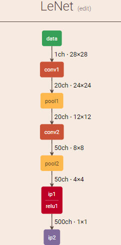
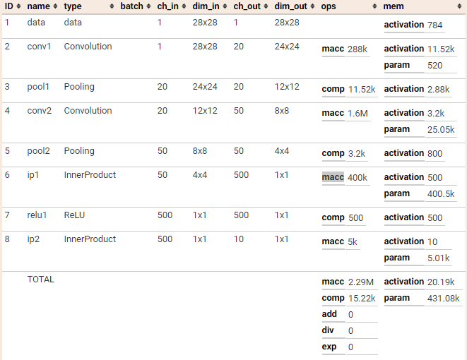
我们可以把网络用 Netscope 工具打开,直接得到结果:
import tensorflow as tf
from tensorflow.examples.tutorials.mnist import input_data
# ================================================================ #
# Train a Sample Model #
# ================================================================ #
# 1. create data
mnist = input_data.read_data_sets('../MNIST', one_hot=True)
with tf.variable_scope('Input'):
tf_x = tf.placeholder(dtype=tf.float32, shape=[None, 28 * 28], name='x')
image = tf.reshape(tf_x, [-1, 28, 28, 1], name='image')
tf_y = tf.placeholder(dtype=tf.float32, shape=[None, 10], name='y')
is_training = tf.placeholder(dtype=tf.bool, shape=None)
# 2. define Network
with tf.variable_scope('Net'):
"""
"SAME" 类型的padding:
out_height = ceil(in_height / strides[1]); ceil向上取整
out_width = ceil(in_width / strides[2])
"VALID"类型的padding:
out_height = ceil((in_height - filter_height + 1) / striders[1])
out_width = ceil((in_width - filter_width + 1) / striders[2]
"""
conv1 = tf.layers.conv2d(inputs=image, filters=20, kernel_size=5,
strides=1, padding='valid', activation=None, name='conv1') # 20x24x24
pool1 = tf.layers.max_pooling2d(inputs=conv1, pool_size=2, strides=2, name='pool1') # 20x12x12
conv2 = tf.layers.conv2d(pool1, 50, 5, 1, 'valid', activation=None, name='conv2') # 50x8x8
pool2 = tf.layers.max_pooling2d(conv2, 2, 2, name='pool2') # 50x4x4
pool2_flat = tf.reshape(pool2, [-1, 4 * 4 * 50])
fc1 = tf.layers.dense(pool2_flat, 500, tf.nn.relu, name='ip1') # 500
predict = tf.layers.dense(fc1, 10, name='ip2') # 10
# 3. define loss & accuracy
with tf.name_scope('loss'):
loss = tf.losses.softmax_cross_entropy(onehot_labels=tf_y, logits=predict, label_smoothing=0.01)
with tf.name_scope('accuracy'):
# tf.metrics.accuracy() 返回 累计[上次的平均accuracy, 这次的平均accuracy]
accuracy = tf.metrics.accuracy(labels=tf.argmax(tf_y, axis=1), predictions=tf.argmax(predict, axis=1))[1]
# 4. define optimizer
with tf.name_scope('train'):
optimizer_op = tf.train.AdamOptimizer(1e-4).minimize(loss)
# 5. initialize
init_op = tf.group(tf.global_variables_initializer(), tf.local_variables_initializer())
# 6.train
saver = tf.train.Saver()
save_path = './leNet_mnist.ckpt'
with tf.Session() as sess:
sess.run(init_op)
for step in range(11000):
"""
mnist.train.num_examples=55000
11000*100/mnist.train.num_examples=20epochs
"""
batch_x, batch_y = mnist.train.next_batch(100)
_, ls = sess.run([optimizer_op, loss],
feed_dict={tf_x: batch_x, tf_y: batch_y, is_training: True})
if step % 100 == 0:
acc_test = sess.run(accuracy,
feed_dict={tf_x: mnist.test.images, tf_y: mnist.test.labels,
is_training: False})
print('Step: ', step, ' | train loss: {:.4f} | test accuracy: {:.3f}'.format(ls, acc_test))
sess.run(tf.local_variables_initializer()) # 不加上这句的话 accuracy 就是个累积平均值了
saver.save(sess, save_path)
# 7.test
with tf.Session() as sess:
sess.run(init_op)
saver.restore(sess, save_path)
acc_test = sess.run(accuracy, feed_dict={tf_x: mnist.test.images,
tf_y: mnist.test.labels,
is_training: False})
print('test accuracy: {}'.format(acc_test)) # test accuracy: 0.991100013256073
View Code
训练得到示例模型 LeNet_mnist.ckpt, 随后为了确定输出节点(Net/ip2/BiasAdd),我们需要到 tensorboard 里去瞅瞅
from tensorflow.summary import FileWriter
sess = tf.Session()
tf.train.import_meta_graph("leNet_mnist.ckpta")
FileWriter("__tb", sess.graph)
View Code
知道了输出节点我们就可以将模型转换成 pb 文件了并计算 FLOPs 了:
# ================================================================ #
# Convert ckpt to pb & Compute FLOPs #
# ================================================================ #
from tensorflow.python.framework import graph_util
def stats_graph(graph):
flops = tf.profiler.profile(graph, options=tf.profiler.ProfileOptionBuilder.float_operation())
params = tf.profiler.profile(graph, options=tf.profiler.ProfileOptionBuilder.trainable_variables_parameter())
print('FLOPs: {}; Trainable params: {}'.format(flops.total_float_ops, params.total_parameters))
with tf.Graph().as_default() as graph:
# 1. Create Graph
image = tf.Variable(initial_value=tf.random_normal([1, 28, 28, 1]))
conv1 = tf.layers.conv2d(inputs=image, filters=20, kernel_size=5,
strides=1, padding='valid', activation=None, name='conv1') # 20x24x24
pool1 = tf.layers.max_pooling2d(inputs=conv1, pool_size=2, strides=2, name='pool1') # 20x12x12
conv2 = tf.layers.conv2d(pool1, 50, 5, 1, 'valid', activation=None, name='conv2') # 50x8x8
pool2 = tf.layers.max_pooling2d(conv2, 2, 2, name='pool2') # 50x4x4
pool2_flat = tf.reshape(pool2, [-1, 4 * 4 * 50])
fc1 = tf.layers.dense(pool2_flat, 500, tf.nn.relu, name='ip1') # 500
predict = tf.layers.dense(fc1, 10, name='ip2') # 10
print('stats before freezing')
stats_graph(graph)
# 2. Freeze Graph
with tf.Session() as sess:
sess.run(tf.global_variables_initializer())
output_graph = graph_util.convert_variables_to_constants(sess, graph.as_graph_def(), ['ip2/BiasAdd'])
with tf.gfile.GFile('LeNet_mnist.pb', "wb") as f:
f.write(output_graph.SerializeToString())
def load_pb(pb):
with tf.gfile.GFile(pb, "rb") as f:
graph_def = tf.GraphDef()
graph_def.ParseFromString(f.read())
with tf.Graph().as_default() as graph:
tf.import_graph_def(graph_def, name='')
return graph
# 3. Load Frozen Graph
graph = load_pb('LeNet_mnist.pb')
print('stats after freezing')
stats_graph(graph)
View Code
stats before freezingFLOPs: 5478522; Trainable params: 431864stats after freezingFLOPs: 4615950; Trainable params: 0 具体的: node name | # parameters _TFProfRoot (--/431.86k params) Variable (1x28x28x1, 784/784 params) conv1 (--/520 params) conv1/bias (20, 20/20 params) conv1/kernel (5x5x1x20, 500/500 params) conv2 (--/25.05k params) conv2/bias (50, 50/50 params) conv2/kernel (5x5x20x50, 25.00k/25.00k params) ip1 (--/400.50k params) ip1/bias (500, 500/500 params) ip1/kernel (800x500, 400.00k/400.00k params) ip2 (--/5.01k params) ip2/bias (10, 10/10 params) ip2/kernel (500x10, 5.00k/5.00k params) node name | # float_ops _TFProfRoot (--/4.62m flops) conv2/Conv2D (3.20m/3.20m flops) ip1/MatMul (800.00k/800.00k flops) conv1/Conv2D (576.00k/576.00k flops) conv1/BiasAdd (11.52k/11.52k flops) pool1/MaxPool (11.52k/11.52k flops) ip2/MatMul (10.00k/10.00k flops) conv2/BiasAdd (3.20k/3.20k flops) pool2/MaxPool (3.20k/3.20k flops) ip1/BiasAdd (500/500 flops) ip2/BiasAdd (10/10 flops) PyTorch
import torch
import torchvision
import torch.nn as nn
import torch.nn.functional as F
import torchvision.transforms as transforms
from torchsummary import summary
# Device configuration
device = torch.device('cpu') #torch.device('cuda: 0' if torch.cuda.is_available() else 'cup')
print(device, torch.__version__)
# Hyper parameters
num_epochs = 5
num_classes = 10
batch_size = 100
learning_rate = 0.01
# MINST DATASET
train_dataset = torchvision.datasets.MNIST(root='H:/Other_Datasets/',
train=True,
transform=transforms.ToTensor(),
download=True)
test_dataset = torchvision.datasets.MNIST(root='H:/Other_Datasets/',
train=False,
transform=transforms.ToTensor())
# Data loader
train_loader = torch.utils.data.DataLoader(dataset=train_dataset,
batch_size=batch_size,
shuffle=True)
test_loader = torch.utils.data.DataLoader(dataset=test_dataset,
batch_size=batch_size,
shuffle=False)
class LeNet(nn.Module):
def __init__(self, in_channels, num_classes):
super(LeNet, self).__init__()
self.conv1 = nn.Conv2d(in_channels, 20, kernel_size=5, stride=1) # 20x24x24
self.pool1 = nn.MaxPool2d(kernel_size=2, stride=2) # 20x12x12
self.conv2 = nn.Conv2d(20, 50, kernel_size=5, stride=1) # 50x8x8
self.pool2 = nn.MaxPool2d(kernel_size=2, stride=2) # 50x4x4
self.fc1 = nn.Linear(50 * 4 * 4, 500) # 500
self.fc2 = nn.Linear(500, num_classes) # 10
def forward(self, input):
out = self.conv1(input)
out = self.pool1(out)
out = self.conv2(out)
out = self.pool2(out)
out = out.reshape(out.size(0), -1) # pytorch folow NCHW convention
out = F.relu(self.fc1(out))
out = self.fc2(out)
return out
model = LeNet(1, num_classes).to(device)
View Code
可直接使用 torchsummary 模块统计参数量 summary(model, (1, 28, 28), device=device.type) """ ---------------------------------------------------------------- Layer (type) Output Shape Param # ================================================================ Conv2d-1 [-1, 20, 24, 24] 520 MaxPool2d-2 [-1, 20, 12, 12] 0 Conv2d-3 [-1, 50, 8, 8] 25,050 MaxPool2d-4 [-1, 50, 4, 4] 0 Linear-5 [-1, 500] 400,500 Linear-6 [-1, 10] 5,010 ================================================================ Total params: 431,080 Trainable params: 431,080 Non-trainable params: 0 ---------------------------------------------------------------- Input size (MB): 0.00 Forward/backward pass size (MB): 0.14 Params size (MB): 1.64 Estimated Total Size (MB): 1.79 ---------------------------------------------------------------- """也可用变体版本 torchscan from torchscan import summary summary(model, (1, 28, 28)) """ __________________________________________________________________________________________ Layer Type Output Shape Param # ========================================================================================== lenet LeNet (-1, 10) 0 ├─conv1 Conv2d (-1, 20, 24, 24) 520 ├─pool1 MaxPool2d (-1, 20, 12, 12) 0 ├─conv2 Conv2d (-1, 50, 8, 8) 25,050 ├─pool2 MaxPool2d (-1, 50, 4, 4) 0 ├─fc1 Linear (-1, 500) 400,500 ├─fc2 Linear (-1, 10) 5,010 ========================================================================================== Trainable params: 431,080 Non-trainable params: 0 Total params: 431,080 ------------------------------------------------------------------------------------------ Model size (params + buffers): 1.64 Mb Framework & CUDA overhead: 0.00 Mb Total RAM usage: 1.64 Mb ------------------------------------------------------------------------------------------ Floating Point Operations on forward: 4.59 MFLOPs Multiply-Accumulations on forward: 2.30 MMACs Direct memory accesses on forward: 2.35 MDMAs __________________________________________________________________________________________ """ 1. 使用开源工具 pytorch-OpCounter (推荐) from thop import profile input = torch.randn(1, 1, 28, 28) macs, params = profile(model, inputs=(input, )) print('Total macc:{}, Total params: {}'.format(macs, params)) """ Total macc:2307720.0, Total params: 431080.0 """ 2. 使用开源工具 torchstat from torchstat import stat stat(model, (1, 28, 28)) """ module name input shape output shape params memory(MB) MAdd Flops MemRead(B) MemWrite(B) duration[%] MemR+W(B) 0 conv1 1 28 28 20 24 24 520.0 0.04 576,000.0 299,520.0 5216.0 46080.0 99.99% 51296.0 1 pool1 20 24 24 20 12 12 0.0 0.01 8,640.0 11,520.0 46080.0 11520.0 0.00% 57600.0 2 conv2 20 12 12 50 8 8 25050.0 0.01 3,200,000.0 1,603,200.0 111720.0 12800.0 0.00% 124520.0 3 pool2 50 8 8 50 4 4 0.0 0.00 2,400.0 3,200.0 12800.0 3200.0 0.00% 16000.0 4 fc1 800 500 400500.0 0.00 799,500.0 400,000.0 1605200.0 2000.0 0.00% 1607200.0 5 fc2 500 10 5010.0 0.00 9,990.0 5,000.0 22040.0 40.0 0.00% 22080.0 total 431080.0 0.07 4,596,530.0 2,322,440.0 22040.0 40.0 99.99% 1878696.0 ========================================================================================================================================== Total params: 431,080 ------------------------------------------------------------------------------------------------------------------------------------------ Total memory: 0.07MB Total MAdd: 4.6MMAdd Total Flops: 2.32MFlops Total MemR+W: 1.79MB """不过,貌似这里和论文中的计算方式不一样,感觉上 conv = macc/2 + bias_op, fc = macc, pool 对于 caffe 的 comp ps: 网上有评论说 MAdd 和 Flops 应该对调! |
【本文地址】