深度学习笔记:卷积神经网络的可视化 |
您所在的位置:网站首页 › 特征化是什么意思 › 深度学习笔记:卷积神经网络的可视化 |
深度学习笔记:卷积神经网络的可视化
|
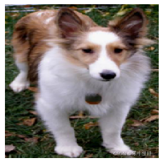
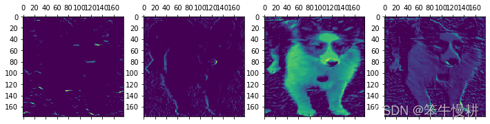
目录 1. 前言 2. 模型的训练 3. 特征图可视化 3.1 加载保存的模型¶ 3.2 图像预处理:将图像转换为张量 3.3 例化一个模型用于返回各层激活输出(即feature map) 3.5 各层各通道汇总可视化 4. 小结 参考文献 1. 前言人们常说,深度学习模型是“黑盒”,即模型学到的东西对于人类来说很难理解。对于很多深度学习模型来说的确是这样的,但是对于卷积神经网络(CNN)却并不尽然。CNN学习到的东西非常适合于可视化,因为它就是学习关于视觉概念的表示!自CNN诞生以来,人们已经开发了很多种技术来对卷积神经网络学习到的东西进行可视化和解释。其中最容易理解也最有用是以下三种: 特征图的可视化。特征图即中间激活层的输出。这个有助于理解CNN的各层如何对输入进行变换,也有助于初步了解CNN中每个过滤器的含义过滤器的可视化。有助于精确理解CNN中每个过滤器对应的视觉模式或视觉概念热力图的可视化。将图像中类激活的热力图可视化有助于理解图像的哪个部分被识别为属于哪个类别,从而可以定位图像中的物体本篇我们先看看特征图的可视化。 特征图的可视化,是指对于给定输入图像,展示模型处理后的各中间层(包括卷积层和池化层等)输出的特征图(各中间层的激活函数的输出代表该层特征图)。这让我们可以看到输入数据在网络中是如何被分解,不同滤波器分别聚焦于原始图像的什么方面的信息。我们希望在三个维度对特征图进行可视化:宽度、高度和深度(通道,channel)。每个通道都对应相对独立的特征。所以将这些特征图可视化的正确方法是将每个通道的内容分别会支持成二维图像。 2. 模型的训练采用之前训练过的一个模型,参见“”。事实上,如果在之前的训练中把这个模型存储下来了的话,可以直接加载已存储的模型而不必重复训练。这个把数据处理到模型训练的代码重新贴一遍只是为了保持本文自身的完备性。详细解说可以参考:利用数据增强在小数据集上从头训练卷积神经网络 import tensorflow as tf from tensorflow import keras from tensorflow.keras import layers from tensorflow.keras import utils import numpy as np import matplotlib.pyplot as plt from PIL import Image print(tf.__version__)数据集准备 def make_subset(subset_name, start_index, end_index): for category in ("cat", "dog"): dir = new_base_dir / subset_name / category src_dir = original_dir / category print(dir) os.makedirs(dir) fnames = [f"{i}.jpg" for i in range(start_index, end_index)] for fname in fnames: shutil.copyfile(src=src_dir / fname, dst=dir / fname) import os, shutil, pathlib original_dir = pathlib.Path("F:\DL\cats-vs-dogs") new_base_dir = pathlib.Path("F:\DL\cats_vs_dogs_small") #print(original_dir, new_base_dir) start_index = np.random.randint(0,8000) end_index = start_index + 1000 start_index3 = end_index end_index3 = start_index3 + 500 if os.path.exists(new_base_dir): shutil.rmtree(new_base_dir) make_subset("train", start_index=start_index, end_index=end_index) make_subset("test", start_index=start_index3, end_index=end_index3)模型搭建 inputs = keras.Input(shape=(180, 180, 3)) x = layers.Conv2D(filters=32, kernel_size=3, activation="relu")(inputs) x = layers.MaxPooling2D(pool_size=2)(x) x = layers.Conv2D(filters=64, kernel_size=3, activation="relu")(x) x = layers.MaxPooling2D(pool_size=2)(x) x = layers.Conv2D(filters=128, kernel_size=3, activation="relu")(x) x = layers.MaxPooling2D(pool_size=2)(x) x = layers.Conv2D(filters=256, kernel_size=3, activation="relu")(x) x = layers.MaxPooling2D(pool_size=2)(x) x = layers.Conv2D(filters=256, kernel_size=3, activation="relu")(x) x = layers.Flatten()(x) x = layers.Dropout(0.5)(x) outputs = layers.Dense(1, activation="sigmoid")(x) model = keras.Model(inputs=inputs, outputs=outputs) model.summary() # Configuring the model for training model.compile(loss="binary_crossentropy",optimizer="rmsprop",metrics=["accuracy"])数据预处理及数据增强 import os from tensorflow.keras.preprocessing.image import ImageDataGenerator batch_size = 32 train_dir = os.path.join('F:\DL\cats_vs_dogs_small', 'train') test_dir = os.path.join('F:\DL\cats_vs_dogs_small', 'test') train_datagen = ImageDataGenerator(rescale=1./255,validation_split=0.3, rotation_range=40, width_shift_range=0.2, height_shift_range=0.2, shear_range=0.2, zoom_range=0.2, horizontal_flip=True, fill_mode='nearest' ) test_datagen = ImageDataGenerator(rescale=1./255) train_generator = train_datagen.flow_from_directory( directory=train_dir, target_size=(180, 180), color_mode="rgb", batch_size=batch_size, class_mode="binary", subset='training', shuffle=True, seed=42 ) valid_generator = train_datagen.flow_from_directory( directory=train_dir, target_size=(180, 180), color_mode="rgb", batch_size=batch_size, class_mode="binary", subset='validation', shuffle=True, seed=42 ) test_generator = test_datagen.flow_from_directory( directory=test_dir, target_size=(180, 180), color_mode="rgb", batch_size=batch_size, class_mode='binary', shuffle=False, seed=42 )模型训练和保存 callbacks = [ keras.callbacks.ModelCheckpoint( filepath="convnet_from_scratch_with_augmentation.keras", save_best_only=True, monitor="val_loss") ] history = model.fit( x = train_generator, validation_data=valid_generator, steps_per_epoch = train_generator.n//train_generator.batch_size, validation_steps = valid_generator.n//valid_generator.batch_size, epochs=100, callbacks=callbacks)训练完以后,大致可以得到在验证集上接近80%的分类准确度。并且训练完的模型被存为文件“convnet_from_scratch_with_augmentation.keras”,以供后续直接加载使用。 3. 特征图可视化 3.1 加载保存的模型¶ model = keras.models.load_model("convnet_from_scratch_with_augmentation.keras") model.summary() 3.2 图像预处理:将图像转换为张量 img_path = "F:/DL/cats-vs-dogs/Dog/24.jpg" def get_img_array(img_path, target_size): img = keras.preprocessing.image.load_img( img_path, target_size=target_size) array = keras.preprocessing.image.img_to_array(img) array = np.expand_dims(array, axis=0) return array img_tensor = get_img_array(img_path, target_size=(180, 180)) print(img_tensor.shape) # Displaying the test picture import matplotlib.pyplot as plt plt.axis("off") plt.imshow(img_tensor[0].astype("uint8")) plt.show() 为了提取想要查看的特征图,我们需要创建一个Keras模型,以图像批量作为输入,并输出所有卷积层和池化层的激活。为此,我们需要使用Keras的Model类,模型的实例化需要两个参数,一个是输入张量(或输入张量列表),一个是输出张量(或输出张量列表)。得到的对象就是一个Keras模型,和之前的Sequential模型一样,将特定输入映射为特定输出。Model类运行多个输出,这个和Sequential类不同。 以下模型接收一张图像输入,将返回原始模型所有各卷积层和池化层的输出。可以理解为这个模型就是原有模型的一个wrapper(套了一层皮),这样我们就可以方便地将所有想观测的中间信息全部引出来。其中,由语句“isinstance(layer, (layers.Conv2D, layers.MaxPooling2D))”进行过滤提取卷积层和池化层。实际上,池化层的输出应该与其前面的卷积层输出大同小异,所以在以下代码将池化层也滤除掉了。 from tensorflow.keras import layers layer_outputs = [] layer_names = [] for layer in model.layers: #if isinstance(layer, (layers.Conv2D, layers.MaxPooling2D)): if isinstance(layer, layers.Conv2D): layer_outputs.append(layer.output) layer_names.append(layer.name) activation_model = keras.Model(inputs=model.input, outputs=layer_outputs) print('There are totally {} layers in this model'.format(len(layer_names)))原始模型总共有13层,其中有5层卷积层和4层池化层。 使用这个模型计算并输出中间层输出,看看第一个卷积层输出的几个通道的数据的显示效果。 import matplotlib.pyplot as plt activations = activation_model.predict(img_tensor) # 确认输出结果的shape与前面model.summary()给出的信息是一致的 first_layer_activation = activations[0] print(first_layer_activation.shape) fig, ax = plt.subplots(1,4,figsize=(12,16)) ax[0].matshow(first_layer_activation[0, :, :, 0], cmap="viridis") ax[1].matshow(first_layer_activation[0, :, :, 5], cmap="viridis") ax[2].matshow(first_layer_activation[0, :, :, 11], cmap="viridis") ax[3].matshow(first_layer_activation[0, :, :, 24], cmap="viridis")
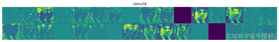
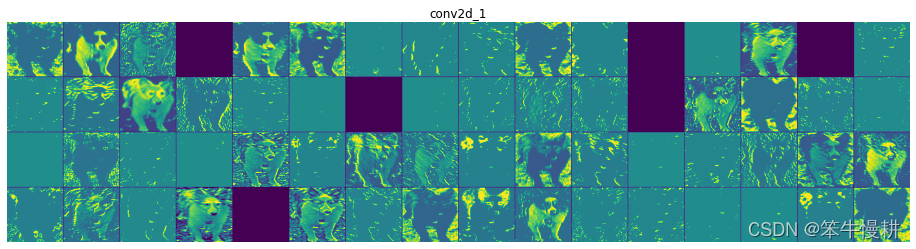
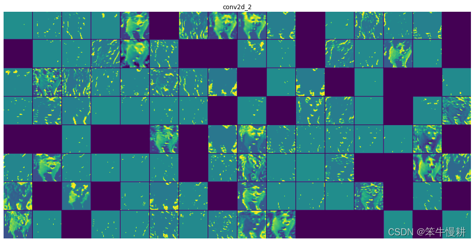
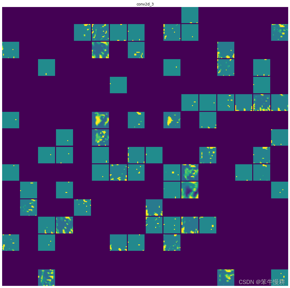
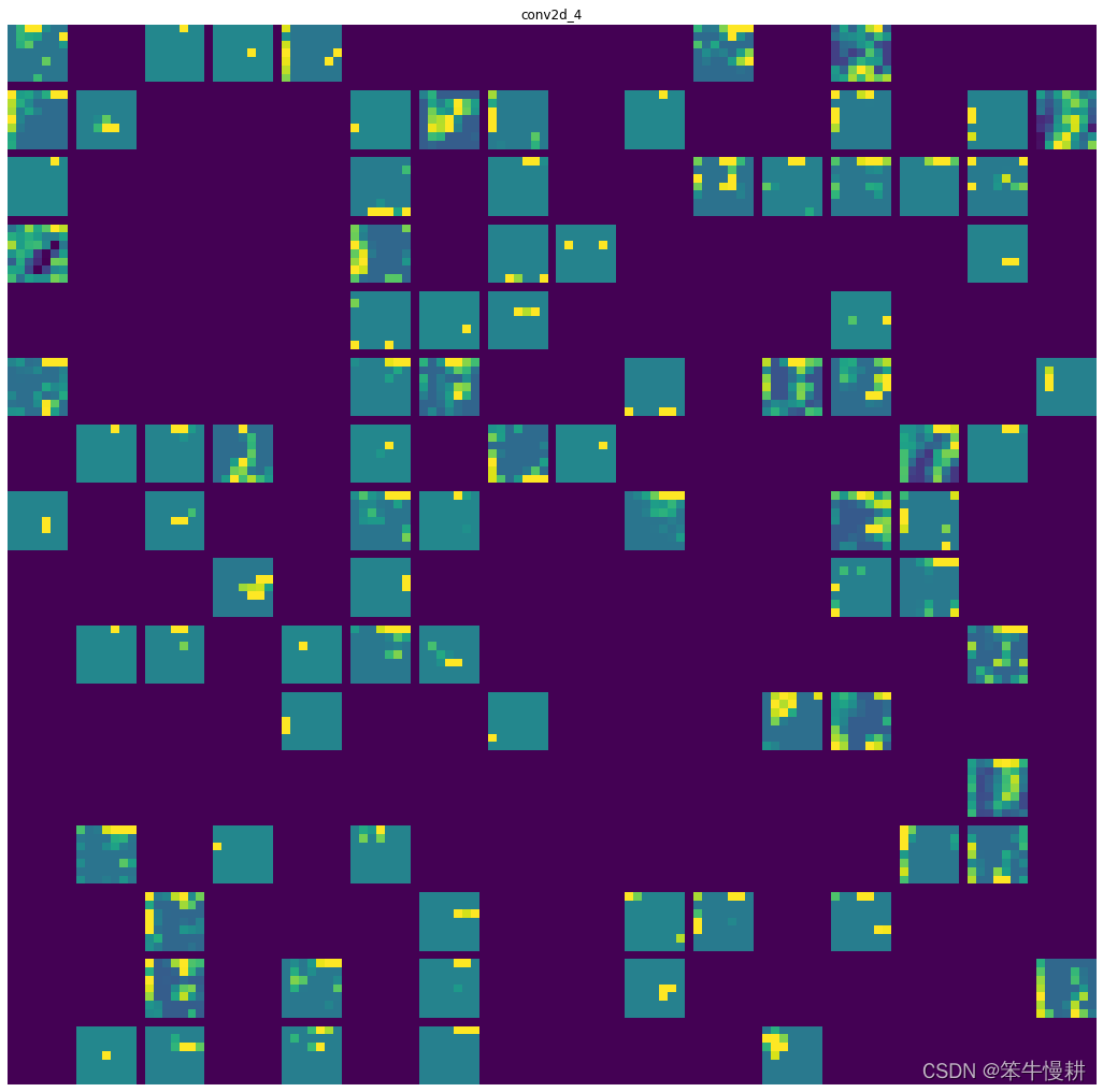
以下代码将所有各层的各个通道的输出均以二维图像的方式汇总画出。 images_per_row = 16 # 每行16个小图 for layer_name, layer_activation in zip(layer_names, activations): print(layer_name) n_features = layer_activation.shape[-1] # Number of features, i.e, channels of the current layer output. size = layer_activation.shape[1] n_cols = n_features // images_per_row # n_cols should be 'number of plots per column', i.e, number of rows. display_grid = np.zeros(((size + 1) * n_cols - 1,images_per_row * (size + 1) - 1)) for col in range(n_cols): for row in range(images_per_row): channel_index = col * images_per_row + row channel_image = layer_activation[0, :, :, channel_index].copy() if channel_image.sum() != 0: #数据处理,使其适合于作为图像展示 channel_image -= channel_image.mean() channel_image /= channel_image.std() channel_image *= 64 channel_image += 128 channel_image = np.clip(channel_image, 0, 255).astype("uint8") display_grid[ col * (size + 1): (col + 1) * size + col, row * (size + 1) : (row + 1) * size + row] = channel_image scale = 1. / size plt.figure(figsize=(scale * display_grid.shape[1], scale * display_grid.shape[0])) plt.title(layer_name) plt.grid(False) plt.axis("off") plt.imshow(display_grid, aspect="auto", cmap="viridis") 输出结果如下所示:
从以上结果中可以看出: 第一层是各种边缘检测器的集合,在这一阶段,激活输出几乎保留了原始图像的所有信息随着层数的加深,激活输出变得越来越抽象。conv2d_3的输出已经超出了人类直观理解的范围。可以这样理解,随着层数的加深,关于图像视觉内容信息越来越少,而关于类别的信息就越来越多激活的稀疏度(sparsity)随着层数的加深而增大。在第一层中,所有滤波器都被输入图像所激活(体现为对应通道有有效的图像信息),而随着层数加深,越来越多的通道对应的图示为空,表明没有被激活,即输入图像中没有找到这些过滤器所习得(编码)的模式。 4. 小结以上实验揭示了深度神经网络学到的表示的一个重要的普遍特征:随着层数的加深,层所提取的特征变得越来越抽象,关于特定输入的信息越来越少,而关于目标的信息则越来越多(本例中即图像的类别:猫和狗)。深度神经网络可以有效地作为信息整流管道(information distillation pipeline),输入原始数据(本例中是RGB信息),反复对其进行变换,将无关信息过滤掉(比如他,图像的具体外观),并放大和细化有用的信息(比如与图像类别有关的信息)。这与人类和动物感知世界的方式类似:人类观察一个场景几秒钟后,可以记住其中有哪些抽象物体(比如说自行车、数或者是哪个人),但是却不一定能记住物体的具体外观。事实上,尽管你可能见过成百上千辆自行车,但是要你试着画一辆自行车出来,估计会是歪歪扭扭的,只具备勉强能让人识别出是自行车的框架性特征。人类的大脑已经学会将视觉输入完全抽象化,将其转换为更高层次的视觉概念,同时过滤掉不想管的视觉细节,这使得大脑很难记住周围事物的具体外观特征。事实上,这也可能是一个明智的自然进化选择。 参考文献[1] Francois Chollet, Deep Learning with Python, Chapter5.4 |
【本文地址】