数字图像处理学习(1) |
您所在的位置:网站首页 › 照片插值放大 › 数字图像处理学习(1) |
数字图像处理学习(1)
|
数字图像处理学习(1)——图像插值Python代码实现
1. 图像插值 (Image Interpolation)2. 最近邻插值法2.1 最近邻插值法2.2 最近邻插值法(Python 代码实现——图像缩小)2.3 运行结果示例
3. 双线性插值法3.1 双线性插值法3.2 双线性插值法(Python代码实现——图片放大)3.3 结果展示
最近在学习数字图像处理,打算长期记录下来。 1. 图像插值 (Image Interpolation)当我们需要放大或者缩小一张数字图像的时候,我们所进行的操作称之为Image Interpolation。 例如:把一张 275*185 的图像转化为原图的一半大小,如下:
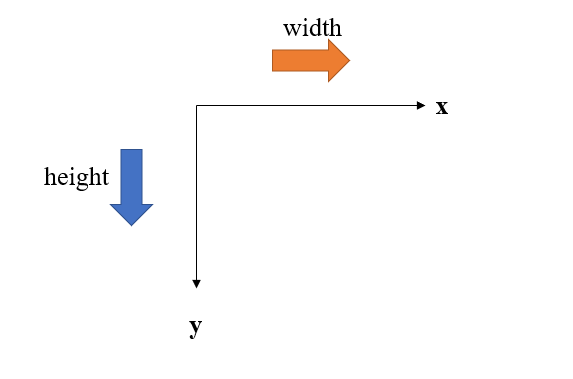
实际上就是根据原来的图片中,所有像素点,按照某种关系在新的图片当中进行 pixel填充的一种操作,这种操作最常见的有几种方法: 最近邻插值法(Nearest Neighbor Interpolation)双线性插值法(bilinear interpolation)双三次插值法(bicubic interpolation)在介绍方法之前,我先总结下个人对图像插值整体思路描述,可以分为4步曲: 读取图片选定插值算法pixel 填充新图片保存 2. 最近邻插值法 2.1 最近邻插值法这是最简单、易懂的一种方法。 设原图片的大小为 ( h e i g h t , w i d t h ) (height, width) (height,width), 图片中某一个像素点的位置为 ( s r c x , s r c y ) (srcx, srcy) (srcx,srcy) 目标图片的大小为
(
d
e
s
h
e
i
g
h
t
,
d
e
s
w
i
d
t
h
)
(desheight, deswidth)
(desheight,deswidth). 目标图片中某一个像素点的位置为
(
d
e
s
x
,
d
e
s
y
)
(desx, desy)
(desx,desy)。 根据等比例关系,易得如下关系: s r c x = d e s x ⋅ ( w i d t h / d e s w i d t h ) srcx=desx·(width/deswidth) srcx=desx⋅(width/deswidth) s r c y = d e s y ⋅ ( h e i g h t / d e s h e i g h t ) srcy=desy·(height/desheight) srcy=desy⋅(height/desheight) 其中会遇到小数的值,那么则一般可以设置四舍五入的方式取整,选择位置。 2.2 最近邻插值法(Python 代码实现——图像缩小) #!/usr/bin/env python # encoding: utf-8 """ @author: H @software: Pycharm @file: ImageInterpolation.py @time: 2020/10/16 8:28 """ import os import numpy as np from PIL import Image file_path = r'D:\postgraduate\first_year\数字图像处理\作业\homework1\practice1\image\jerry.jpg' img = Image.open(file_path) # 读取图片,格式为Image # 把Image格式的图片转化为numpy格式进性图像处理 img = np.array(img, dtype=np.uint8) height, width, mode = img.shape[0], img.shape[1], img.shape[2] # 取出高、宽、通道数 print(height, width, mode) # (275 183 3) # 缩放的目标大小,这里以缩放为原图的1/2为例 desWidth = int(width * 0.5) desHeight = int(height * 0.5) desImage = np.zeros((desHeight, desWidth, mode), np.uint8) # 定义一个目标图片代表的array,纯黑图片 # 像素填充 # 方法1:最近邻插值法 for des_x in range(0, desHeight): for des_y in range(0, desWidth): # 判断新像素点在原图中的像素点坐标 src_x = int(des_x * (height/desHeight)) src_y = int(des_y * (width/desWidth)) desImage[des_x, des_y] = img[src_x, src_y] # 填充 print(desImage.shape) des_img = Image.fromarray(desImage) des_img.save('./image/jerry.jpg') # 图片另存为 2.3 运行结果示例
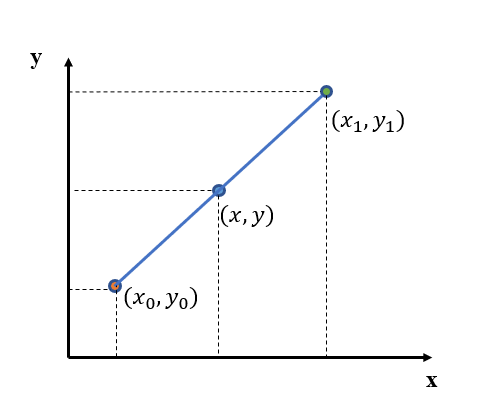
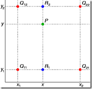
在介绍双线性插值之前,我们需要知道单线性插值的概念。 已知要求点 ( x , y ) (x,y) (x,y)某一条直线上(某一维度),其他两个点坐标为: ( x 0 , y 0 ) (x_0,y_0) (x0,y0), ( x 1 , y 1 ) (x_1,y_1) (x1,y1) 其中
y
y
y 是关于
x
x
x 的某种函数,根据
x
x
x 计算出
x
x
x 对应的像素值
y
y
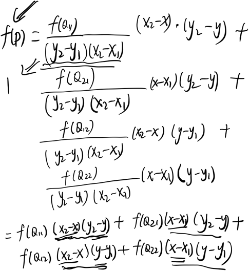
y 总结为: f ( x ) = x 1 − x x 1 − x 0 ⋅ f ( x 0 ) + x − x 0 x 1 − x 0 ⋅ f ( x 1 ) f(x)=\frac{x_1-x}{x_1-x_0}·f(x_0)+\frac{x-x_0}{x_1-x_0}·f(x_1) f(x)=x1−x0x1−x⋅f(x0)+x1−x0x−x0⋅f(x1) 双线性插值法实际上就是进行了两个维度的单线性插值。可分为: 两次水平方向的单线性插值( x x x 轴)根据 x x x 的结果进行一次垂直方向的单线性插值( y y y 轴)当然 x x x 和 y y y 可以互换。 这是找的一张比较经典的图: 结合单线性插值的结论,可以进行如下运算: ① 两次 x x x 轴的线性插值 f ( R 1 ) = x 2 − x x 2 − x 1 ⋅ f ( Q 11 ) + x − x 1 x 2 − x 1 ⋅ f ( Q 21 ) f(R_1)=\frac{x_2-x}{x_2-x_1}·f(Q_{11})+\frac{x-x_1}{x_2-x_1}·f(Q_{21}) f(R1)=x2−x1x2−x⋅f(Q11)+x2−x1x−x1⋅f(Q21) f ( R 2 ) = x 2 − x x 2 − x 1 ⋅ f ( Q 12 ) + x − x 1 x 2 − x 1 ⋅ f ( Q 22 ) f(R_2)=\frac{x_2-x}{x_2-x_1}·f(Q_{12})+\frac{x-x_1}{x_2-x_1}·f(Q_{22}) f(R2)=x2−x1x2−x⋅f(Q12)+x2−x1x−x1⋅f(Q22) ② 进行一次 y y y 轴的线性插值 f ( P ) = y 2 − y y 2 − y 1 ⋅ f ( R 1 ) + y − y 1 y 2 − y 1 ⋅ f ( R 2 ) f(P)=\frac{y_2-y}{y_2-y_1}·f(R_1)+\frac{y-y_1}{y_2-y_1}·f(R_{2}) f(P)=y2−y1y2−y⋅f(R1)+y2−y1y−y1⋅f(R2) 联合① ②两式(害,偷个懒直接上才草稿),可得:
像这张放大的图片的男人一样,加油加油! |


 可以得出:
可以得出: 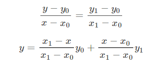 这个结果就好比,一条直线上的两个磁铁,对中间的铁块的力的作用的矢量叠加(不考虑方向)。


【本文地址】
今日新闻 |
推荐新闻 |