在拓扑优化中的灵敏度滤波和密度滤波有什么区别? |
您所在的位置:网站首页 › 灵敏度成器 › 在拓扑优化中的灵敏度滤波和密度滤波有什么区别? |
在拓扑优化中的灵敏度滤波和密度滤波有什么区别?
88行代码中的解释 经典的文章:《Efficient topology optimization in MATLAB using 88 lines of code》
 图1 page3 图1 page3  图2 page4 这篇文章中关于这个问题的描述 为了确定在优化过程中解的存在并且避免棋盘格效应而采用灵敏度或密度滤波的方式。
88行代码
%%%% AN 88 LINE TOPOLOGY OPTIMIZATION CODE Nov, 2010 %%%%
function [x]=top88(nelx,nely,volfrac,penal,rmin,ft)
%% MATERIAL PROPERTIES 材料属性
nelx=5;nely=5;volfrac=0.5;penal=3;rmin=2.1;ft=2;
E0 = 1;
Emin = 1e-9;
nu = 0.3;
%% PREPARE FINITE ELEMENT ANALYSIS 准备有限元分析
A11 = [12 3 -6 -3; 3 12 3 0; -6 3 12 -3; -3 0 -3 12];
A12 = [-6 -3 0 3; -3 -6 -3 -6; 0 -3 -6 3; 3 -6 3 -6];
B11 = [-4 3 -2 9; 3 -4 -9 4; -2 -9 -4 -3; 9 4 -3 -4];
B12 = [ 2 -3 4 -9; -3 2 9 -2; 4 9 2 3; -9 -2 3 2];
KE = 1/(1-nu^2)/24*([A11 A12;A12' A11]+nu*[B11 B12;B12' B11]);
nodenrs = reshape(1:(1+nelx)*(1+nely),1+nely,1+nelx);%reshape 矩阵重构
edofVec = reshape(2*nodenrs(1:end-1,1:end-1)+1,nelx*nely,1);%end表示最后一行 或 最后一列
edofMat = repmat(edofVec,1,8)+repmat([0 1 2*nely+[2 3 0 1] -2 -1],nelx*nely,1);%repmat 矩阵重复 矩阵元素刚度有效的装配到全局刚度矩阵中 矩阵的第i行代表第i个元素的8个自由度指标
iK = reshape(kron(edofMat,ones(8,1))',64*nelx*nely,1);%行索引
jK = reshape(kron(edofMat,ones(1,8))',64*nelx*nely,1);%列索引
% DEFINE LOADS AND SUPPORTS (HALF MBB-BEAM)
F = sparse(2,1,-1,2*(nely+1)*(nelx+1),1);
U = zeros(2*(nely+1)*(nelx+1),1);
fixeddofs = union([1:2:2*(nely+1)],[2*(nelx+1)*(nely+1)]);
alldofs = [1:2*(nely+1)*(nelx+1)];
freedofs = setdiff(alldofs,fixeddofs);%设置两个矩阵的差集
%% PREPARE FILTER 准备过滤器
iH = ones(nelx*nely*(2*(ceil(rmin)-1)+1)^2,1);
jH = ones(size(iH));
sH = zeros(size(iH));
k = 0;
for i1 = 1:nelx
for j1 = 1:nely
e1 = (i1-1)*nely+j1;
for i2 = max(i1-(ceil(rmin)-1),1):min(i1+(ceil(rmin)-1),nelx)
for j2 = max(j1-(ceil(rmin)-1),1):min(j1+(ceil(rmin)-1),nely)
e2 = (i2-1)*nely+j2;
k = k+1;
iH(k) = e1;
jH(k) = e2;
sH(k) = max(0,rmin-sqrt((i1-i2)^2+(j1-j2)^2));
end
end
end
end
H = sparse(iH,jH,sH);%Hei,
Ha=full(H);
Hs = sum(H,2);%包含每一行总和的列向量求和i∈Ne Hei,
Hsa=full(Hs);
%% INITIALIZE ITERATION 循环初始化
x = repmat(volfrac,nely,nelx);
xPhys = x;
loop = 0;
change = 1;
%% START ITERATION 开始循环
while change > 0.01
loop = loop + 1;
%% FE-ANALYSIS 有限元分析 finite element
sK = reshape(KE(:)*(Emin+xPhys(:)'.^penal*(E0-Emin)),64*nelx*nely,1);
K = sparse(iK,jK,sK);K = (K+K')/2;
U(freedofs) = K(freedofs,freedofs)\F(freedofs);
%% OBJECTIVE FUNCTION AND SENSITIVITY ANALYSIS 目标函数与敏感度分析
ce = reshape(sum((U(edofMat)*KE).*U(edofMat),2),nely,nelx);
c = sum(sum((Emin+xPhys.^penal*(E0-Emin)).*ce));
dc = -penal*(E0-Emin)*xPhys.^(penal-1).*ce;
dv = ones(nely,nelx);
%% FILTERING/MODIFICATION OF SENSITIVITIES 敏感度过滤与修改
if ft == 1
dc(:) = H*(x(:).*dc(:))./Hs./max(1e-3,x(:));%H代表原文中的Hei,Hs代表原文中的Hei的和
elseif ft == 2
dc(:) = H*(dc(:)./Hs);%灵敏度改善
dv(:) = H*(dv(:)./Hs);%灵敏度改善
end
%% OPTIMALITY CRITERIA UPDATE OF DESIGN VARIABLES AND PHYSICAL DENSITIES 优化标准更新设计变量和物理密度 OC法 optimality criteria
l1 = 0; l2 = 1e9; move = 0.2;
while (l2-l1)/(l1+l2) > 1e-3
lmid = 0.5*(l2+l1);
xnew = max(0,max(x-move,min(1,min(x+move,x.*sqrt(-dc./dv/lmid)))));
if ft == 1
xPhys = xnew;
elseif ft == 2
xPhys(:) = (H*xnew(:))./Hs;%密度过滤
end
if sum(xPhys(:)) > volfrac*nelx*nely, l1 = lmid; else l2 = lmid; end
end
change = max(abs(xnew(:)-x(:)));
x = xnew;
%% PRINT RESULTS 打印结果
fprintf(' It.:%5i Obj.:%11.4f Vol.:%7.3f ch.:%7.3f\n',loop,c, ...
mean(xPhys(:)),change);
%% PLOT DENSITIES 画出密度
colormap(gray); imagesc(1-xPhys); caxis([0 1]); axis equal; axis off; drawnow;
end
%
%%%%%%%%%%%%%%%%%%%%%%%%%%%%%%%%%%%%%%%%%%%%%%%%%%%%%%%%%%%%%%%%%%%%%%%%%%%%
% This Matlab code was written by E. Andreassen, A. Clausen, M. Schevenels,%
% B. S. Lazarov and O. Sigmund, Department of Solid Mechanics, %
% Technical University of Denmark, %
% DK-2800 Lyngby, Denmark. %
% Please sent your comments to: [email protected] %
% %
% The code is intended for educational purposes and theoretical details %
% are discussed in the paper %
% "Efficient topology optimization in MATLAB using 88 lines of code, %
% E. Andreassen, A. Clausen, M. Schevenels, %
% B. S. Lazarov and O. Sigmund, Struct Multidisc Optim, 2010 %
% This version is based on earlier 99-line code %
% by Ole Sigmund (2001), Structural and Multidisciplinary Optimization, %
% Vol 21, pp. 120--127. %
% %
% The code as well as a postscript version of the paper can be %
% downloaded from the web-site: http://www.topopt.dtu.dk %
% %
% Disclaimer: %
% The authors reserves all rights but do not guaranty that the code is %
% free from errors. Furthermore, we shall not be liable in any event %
% caused by the use of the program. %
%%%%%%%%%%%%%%%%%%%%%%%%%%%%%%%%%%%%%%%%%%%%%%%%%%%%%%%%%%%%%%%%%%%%%%%%%%%%
密度滤波和灵敏度滤波
if ft == 1
dc(:) = H*(x(:).*dc(:))./Hs./max(1e-3,x(:)); % 完成灵敏度滤波
elseif ft == 2
dc(:) = H*(dc(:)./Hs);% 修正目标函数灵敏度值
dv(:) = H*(dv(:)./Hs);% 修正约束函数灵敏度值
end
if ft == 1
xPhys = xnew;
elseif ft == 2
xPhys(:) = (H*xnew(:))./Hs;%密度过滤
end 图2 page4 这篇文章中关于这个问题的描述 为了确定在优化过程中解的存在并且避免棋盘格效应而采用灵敏度或密度滤波的方式。
88行代码
%%%% AN 88 LINE TOPOLOGY OPTIMIZATION CODE Nov, 2010 %%%%
function [x]=top88(nelx,nely,volfrac,penal,rmin,ft)
%% MATERIAL PROPERTIES 材料属性
nelx=5;nely=5;volfrac=0.5;penal=3;rmin=2.1;ft=2;
E0 = 1;
Emin = 1e-9;
nu = 0.3;
%% PREPARE FINITE ELEMENT ANALYSIS 准备有限元分析
A11 = [12 3 -6 -3; 3 12 3 0; -6 3 12 -3; -3 0 -3 12];
A12 = [-6 -3 0 3; -3 -6 -3 -6; 0 -3 -6 3; 3 -6 3 -6];
B11 = [-4 3 -2 9; 3 -4 -9 4; -2 -9 -4 -3; 9 4 -3 -4];
B12 = [ 2 -3 4 -9; -3 2 9 -2; 4 9 2 3; -9 -2 3 2];
KE = 1/(1-nu^2)/24*([A11 A12;A12' A11]+nu*[B11 B12;B12' B11]);
nodenrs = reshape(1:(1+nelx)*(1+nely),1+nely,1+nelx);%reshape 矩阵重构
edofVec = reshape(2*nodenrs(1:end-1,1:end-1)+1,nelx*nely,1);%end表示最后一行 或 最后一列
edofMat = repmat(edofVec,1,8)+repmat([0 1 2*nely+[2 3 0 1] -2 -1],nelx*nely,1);%repmat 矩阵重复 矩阵元素刚度有效的装配到全局刚度矩阵中 矩阵的第i行代表第i个元素的8个自由度指标
iK = reshape(kron(edofMat,ones(8,1))',64*nelx*nely,1);%行索引
jK = reshape(kron(edofMat,ones(1,8))',64*nelx*nely,1);%列索引
% DEFINE LOADS AND SUPPORTS (HALF MBB-BEAM)
F = sparse(2,1,-1,2*(nely+1)*(nelx+1),1);
U = zeros(2*(nely+1)*(nelx+1),1);
fixeddofs = union([1:2:2*(nely+1)],[2*(nelx+1)*(nely+1)]);
alldofs = [1:2*(nely+1)*(nelx+1)];
freedofs = setdiff(alldofs,fixeddofs);%设置两个矩阵的差集
%% PREPARE FILTER 准备过滤器
iH = ones(nelx*nely*(2*(ceil(rmin)-1)+1)^2,1);
jH = ones(size(iH));
sH = zeros(size(iH));
k = 0;
for i1 = 1:nelx
for j1 = 1:nely
e1 = (i1-1)*nely+j1;
for i2 = max(i1-(ceil(rmin)-1),1):min(i1+(ceil(rmin)-1),nelx)
for j2 = max(j1-(ceil(rmin)-1),1):min(j1+(ceil(rmin)-1),nely)
e2 = (i2-1)*nely+j2;
k = k+1;
iH(k) = e1;
jH(k) = e2;
sH(k) = max(0,rmin-sqrt((i1-i2)^2+(j1-j2)^2));
end
end
end
end
H = sparse(iH,jH,sH);%Hei,
Ha=full(H);
Hs = sum(H,2);%包含每一行总和的列向量求和i∈Ne Hei,
Hsa=full(Hs);
%% INITIALIZE ITERATION 循环初始化
x = repmat(volfrac,nely,nelx);
xPhys = x;
loop = 0;
change = 1;
%% START ITERATION 开始循环
while change > 0.01
loop = loop + 1;
%% FE-ANALYSIS 有限元分析 finite element
sK = reshape(KE(:)*(Emin+xPhys(:)'.^penal*(E0-Emin)),64*nelx*nely,1);
K = sparse(iK,jK,sK);K = (K+K')/2;
U(freedofs) = K(freedofs,freedofs)\F(freedofs);
%% OBJECTIVE FUNCTION AND SENSITIVITY ANALYSIS 目标函数与敏感度分析
ce = reshape(sum((U(edofMat)*KE).*U(edofMat),2),nely,nelx);
c = sum(sum((Emin+xPhys.^penal*(E0-Emin)).*ce));
dc = -penal*(E0-Emin)*xPhys.^(penal-1).*ce;
dv = ones(nely,nelx);
%% FILTERING/MODIFICATION OF SENSITIVITIES 敏感度过滤与修改
if ft == 1
dc(:) = H*(x(:).*dc(:))./Hs./max(1e-3,x(:));%H代表原文中的Hei,Hs代表原文中的Hei的和
elseif ft == 2
dc(:) = H*(dc(:)./Hs);%灵敏度改善
dv(:) = H*(dv(:)./Hs);%灵敏度改善
end
%% OPTIMALITY CRITERIA UPDATE OF DESIGN VARIABLES AND PHYSICAL DENSITIES 优化标准更新设计变量和物理密度 OC法 optimality criteria
l1 = 0; l2 = 1e9; move = 0.2;
while (l2-l1)/(l1+l2) > 1e-3
lmid = 0.5*(l2+l1);
xnew = max(0,max(x-move,min(1,min(x+move,x.*sqrt(-dc./dv/lmid)))));
if ft == 1
xPhys = xnew;
elseif ft == 2
xPhys(:) = (H*xnew(:))./Hs;%密度过滤
end
if sum(xPhys(:)) > volfrac*nelx*nely, l1 = lmid; else l2 = lmid; end
end
change = max(abs(xnew(:)-x(:)));
x = xnew;
%% PRINT RESULTS 打印结果
fprintf(' It.:%5i Obj.:%11.4f Vol.:%7.3f ch.:%7.3f\n',loop,c, ...
mean(xPhys(:)),change);
%% PLOT DENSITIES 画出密度
colormap(gray); imagesc(1-xPhys); caxis([0 1]); axis equal; axis off; drawnow;
end
%
%%%%%%%%%%%%%%%%%%%%%%%%%%%%%%%%%%%%%%%%%%%%%%%%%%%%%%%%%%%%%%%%%%%%%%%%%%%%
% This Matlab code was written by E. Andreassen, A. Clausen, M. Schevenels,%
% B. S. Lazarov and O. Sigmund, Department of Solid Mechanics, %
% Technical University of Denmark, %
% DK-2800 Lyngby, Denmark. %
% Please sent your comments to: [email protected] %
% %
% The code is intended for educational purposes and theoretical details %
% are discussed in the paper %
% "Efficient topology optimization in MATLAB using 88 lines of code, %
% E. Andreassen, A. Clausen, M. Schevenels, %
% B. S. Lazarov and O. Sigmund, Struct Multidisc Optim, 2010 %
% This version is based on earlier 99-line code %
% by Ole Sigmund (2001), Structural and Multidisciplinary Optimization, %
% Vol 21, pp. 120--127. %
% %
% The code as well as a postscript version of the paper can be %
% downloaded from the web-site: http://www.topopt.dtu.dk %
% %
% Disclaimer: %
% The authors reserves all rights but do not guaranty that the code is %
% free from errors. Furthermore, we shall not be liable in any event %
% caused by the use of the program. %
%%%%%%%%%%%%%%%%%%%%%%%%%%%%%%%%%%%%%%%%%%%%%%%%%%%%%%%%%%%%%%%%%%%%%%%%%%%%
密度滤波和灵敏度滤波
if ft == 1
dc(:) = H*(x(:).*dc(:))./Hs./max(1e-3,x(:)); % 完成灵敏度滤波
elseif ft == 2
dc(:) = H*(dc(:)./Hs);% 修正目标函数灵敏度值
dv(:) = H*(dv(:)./Hs);% 修正约束函数灵敏度值
end
if ft == 1
xPhys = xnew;
elseif ft == 2
xPhys(:) = (H*xnew(:))./Hs;%密度过滤
end
ft=1时,灵敏度滤波。设计变量就是单元的伪密度,直接对目标函数的灵敏度进行滤波。 ft=2时,密度滤波。这里分为两步进行,第一步是根据链式法则求解目标函数对设计变量的灵敏度,第二步是对设计变量进行密度滤波,得到单元伪密度。 注意:在该代码中,x代表设计变量,xPhys代表得到的真实物理密度。 灵敏度滤波 %% MATERIAL PROPERTIES 材料属性 nelx=300;nely=100;volfrac=0.5;penal=3;rmin=2.1;ft=1; E0 = 1; Emin = 1e-9; nu = 0.3;Result  Fig.1 x设计变量结果 Fig.1 x设计变量结果
 Fig.1 xPhys设计变量结果
此时求得的目标柔度值为
It.: 100 Obj.: 190.4912 Vol.: 0.500 ch.: 0.200
密度滤波
%% MATERIAL PROPERTIES 材料属性
nelx=300;nely=100;volfrac=0.5;penal=3;rmin=2.1;ft=1;
E0 = 1;
Emin = 1e-9;
nu = 0.3; Fig.1 xPhys设计变量结果
此时求得的目标柔度值为
It.: 100 Obj.: 190.4912 Vol.: 0.500 ch.: 0.200
密度滤波
%% MATERIAL PROPERTIES 材料属性
nelx=300;nely=100;volfrac=0.5;penal=3;rmin=2.1;ft=1;
E0 = 1;
Emin = 1e-9;
nu = 0.3;
Result  Fig.1 x设计变量结果 Fig.1 x设计变量结果
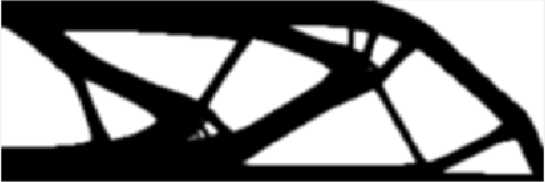 Fig.2 xPhys设计变量结果
此时求得的目标柔度值为
It.: 100 Obj.: 198.1180 Vol.: 0.500 ch.: 0.200 Fig.2 xPhys设计变量结果
此时求得的目标柔度值为
It.: 100 Obj.: 198.1180 Vol.: 0.500 ch.: 0.200
这两种滤波方式所得到的结果稍有不同,但他们最终的结果是一样的,我的猜测是,密度滤波的收敛速度更慢一点。 |
【本文地址】
今日新闻 |
推荐新闻 |