三角函数 |
您所在的位置:网站首页 › 正弦值与角度的计算公式 › 三角函数 |
三角函数
 三角函数图像(动画演示)
三角学 三角函数图像(动画演示)
三角学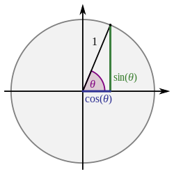 历史(英语:History of trigonometry)
三角函数 (反三角函数)
广义三角函数(英语:Generalized trigonometry)
参考
恒等式
精确值
三角表(英语:Trigonometric tables)
单位圆
定理
正弦
餘弦
正切
餘切
勾股定理
微积分
三角换元法
积分 (反三角函数)
微分
查论编
历史(英语:History of trigonometry)
三角函数 (反三角函数)
广义三角函数(英语:Generalized trigonometry)
参考
恒等式
精确值
三角表(英语:Trigonometric tables)
单位圆
定理
正弦
餘弦
正切
餘切
勾股定理
微积分
三角换元法
积分 (反三角函数)
微分
查论编
三角函数(英語:trigonometric functions[註 1])是數學很常見的一類關於角度的函数。三角函數將直角三角形的内角和它的两邊的比值相关联,亦可以用单位圆的各种有关线段的长的等价來定义。三角函数在研究三角形和圆形等几何形状的性质时有著重要的作用,亦是研究振动、波、天体运动和各种周期性现象的基础数学工具[1]。在数学分析上,三角函数亦定义为无穷级数或特定微分方程的解,允许它们的取值扩展到任意实数值,甚至是複數值。 常見的三角函数有正弦函数( sin {\displaystyle \sin } )、余弦函数( cos {\displaystyle \cos } )和正切函数( tan {\displaystyle \tan } 或 tg {\displaystyle \operatorname {tg} } )[1];在航海学、测绘学和工程学等其他学科中还会用到例如余切函数( cot {\displaystyle \cot } 或 ctg {\displaystyle \operatorname {ctg} } )、正割函数( sec {\displaystyle \sec } )、余割函数( csc {\displaystyle \csc } )、正矢函数和半正矢函数等其它三角函数。不同的三角函数之间的关系可以几何直观或计算得出,称为三角恒等式。 三角函数一般用于计算三角形中的未知长度的边和未知的角度,在导航、工程学和物理学方面都有广泛的用途。另外,以三角函数为模版,可以定义一类相似的函数,叫做双曲函数[2]。常见的双曲函数也称双曲正弦函数、双曲余弦函数等。 目录 1 历史 2 几何定义 2.1 以直角三角形來定义 2.2 以直角坐标系來定义 2.3 单位圆定义 3 基本性质 3.1 三角恒等式 3.2 微积分 4 分析学定义 4.1 級數定義 4.1.1 与指数函数和复数的關系 4.2 较少見的三角函數 4.3 微分方程定义 4.3.1 弧度的重要性 4.4 利用函数方程定义三角函数 5 计算 5.1 三角函数的特殊值 6 反三角函数 7 相关定理 7.1 正弦定理 7.2 余弦定理 7.3 正切定理[24] 7.4 餘切定理 7.5 周期函数 8 参见 9 注释 10 参考资料 11 延伸阅读 12 外部链接 历史[编辑]三角函数的早期研究可以追溯到古代。例如古埃及数学家在鑑別尼羅河泛濫後的土地邊界、保持金字塔每邊斜度相同,都使用了三角術,只是他們可能還沒有對這種方式定名而已。古希腊三角术的奠基人是公元前2世纪的喜帕恰斯。他按照古巴比伦人的做法,将圆周分为360等份(即圆周的弧度为360度,与现代的弧度制不同)。对于指定弧度,他给出了对应的弦的长度数值,这记法和现代的正弦函数等价。喜帕恰斯实际上给出了最早的三角函数数值表。然而古希腊的三角学基本是球面三角学。这与古希腊人研究的主体是天文学有关。梅涅劳斯在他的著作《球面学》中使用了正弦来描述球面的梅涅劳斯定理。古希腊三角学与其天文学的应用在埃及的托勒密时代达到了高峰,托勒密在《数学汇编》(Syntaxis Mathematica)中计算了36度角和72度角的正弦值,还给出了计算和角公式和半角公式的方法。托勒密还给出了所有0到180度的所有整数和半整数弧度对应的正弦值[3]:133-140[4]:151-152。 希腊文化传播到古印度后,印度人繼續研究了三角术。公元5世纪末的数学家阿耶波多提出用弧对应的弦长的一半来对应半弧的正弦,後来古印度数学家亦用了这做法,和现代的正弦定义一致[4]:189。阿耶波多的计算中也使用了余弦和正割。他在计算弦长时使用了不同的单位,重新计算了0到90度中间隔三又四分之三度(3.75°)的三角函数值表[4]:193。然而古印度的数学与当时的中国一样,停留在计算方面,缺乏系统的定义和演绎的证明。阿拉伯人也采用了古印度人的正弦定义,但他们的三角学是直接继承于古希腊。阿拉伯天文学家引入了正切和余切、正割和余割的概念,并计算了间隔10分(10′)的正弦和正切数值表[3]:214-215。到了公元14世纪,阿拉伯人将三角计算重新以算术方式代数化(古希腊人采用的是建立在几何上的推导方式)的努力为後来三角学从天文学中独立出来,成为了有更广泛应用的学科奠定了基础。[3]:225 进入15世纪后,阿拉伯数学文化开始传入欧洲。随着欧洲商业兴盛起來,航行、历法测定和地理测绘中出现了对三角学的需求。在翻译阿拉伯数学著作的同时,欧洲数学家开始制作更详细精确的三角函数值表。哥白尼的学生乔治·约阿希姆·瑞提克斯(英语:Goerg Joachim Rheticus)制作了间隔10秒(10″)的正弦表,有9位精确值。瑞提克斯还改变了正弦的定义,原来称弧对应的弦长是正弦,瑞提克斯则将角度对应的弦长称为正弦。16世纪后,数学家开始将古希腊有关球面三角的结果和定理转化为平面三角定理。弗朗索瓦·韦达给出了托勒密的不少结果对应的平面三角形式。他还尝试计算了多倍角正弦的表达方式。[3]:275-278 18世纪开始引进解析几何等分析学工具,数学家开始用分析学研究三角函数。牛顿在1669年的《分析学》一书中给出了正弦和余弦函数的无穷级数表示。Collins将牛顿的结果告诉詹姆斯·格列高里,後者进一步给出了正切等三角函数的无穷级数。莱布尼兹在1673年左右也独立得到这结果[5]:162-163。欧拉的《无穷小量分析引论》(Introductio in Analysin Infinitorum,1748年)对建立三角函数的分析处理做了最主要的贡献,他定义三角函数为无穷级数,并表述了欧拉公式,还有使用接近现代的简写sin.、cos.、tang.、cot.、sec.和csc.(cosec.)。 1631年徐光启与邓玉函、汤若望合撰《大测》首次将三角函数引入中国并确立了正弦、余弦等译名。 几何定义[编辑] 以直角三角形來定义[编辑] a,b,h分別為角A的对边、邻边和斜边 a,b,h分別為角A的对边、邻边和斜边
直角三角形只有锐角(大小在0至90度之间的角)三角函数的定义[6]。指定锐角 θ {\displaystyle \theta } 可做出直角三角形,使一個内角為 θ {\displaystyle \theta } ,對應股(对边a)、勾(邻边b)和弦(斜边h): θ {\displaystyle \theta } 的正弦是对边与斜边的比值: sin θ = a h {\displaystyle \sin {\theta }={\frac {a}{h}}} θ {\displaystyle \theta } 的餘弦是邻边与斜边的比值: cos θ = b h {\displaystyle \cos {\theta }={\frac {b}{h}}} θ {\displaystyle \theta } 的正切是对边与邻边的比值: tan θ = a b {\displaystyle \tan {\theta }={\frac {a}{b}}} θ {\displaystyle \theta } 的余切是邻边与对边的比值: cot θ = b a {\displaystyle \cot {\theta }={\frac {b}{a}}} θ {\displaystyle \theta } 的正割是斜边与邻边的比值: sec θ = h b {\displaystyle \sec {\theta }={\frac {h}{b}}} θ {\displaystyle \theta } 的餘割是斜边与对边的比值: csc θ = h a {\displaystyle \csc {\theta }={\frac {h}{a}}} 以直角坐标系來定义[编辑]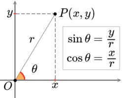
假设 P ( x , y ) {\textstyle P(x,y)} 是平面直角坐标系 x O y {\textstyle xOy} 中的一点, θ {\textstyle \theta } 是横轴正向 O x → {\textstyle {\vec {Ox}}} 逆时针旋转到 O P → {\textstyle {\vec {OP}}} 方向所形成的一個角, r = x 2 + y 2 > 0 {\textstyle r={\sqrt {x^{2}+y^{2}}}>0} 是 P {\textstyle P} 到原点 O {\textstyle O} 的距离,则 θ {\displaystyle \theta } 的六種三角函数定义为[7]: 正弦 餘弦 正切 餘切 正割 餘割 sin θ = y r {\displaystyle \sin \theta ={\frac {y}{r}}} cos θ = x r {\displaystyle \cos \theta ={\frac {x}{r}}} tan θ = y x {\displaystyle \tan \theta ={\frac {y}{x}}} cot θ = x y {\displaystyle \cot \theta ={\frac {x}{y}}} sec θ = r x {\displaystyle \sec \theta ={\frac {r}{x}}} csc θ = r y {\displaystyle \csc \theta ={\frac {r}{y}}}这样可以定义任何角度的三角函数(除非当定义式无意义时)。大于360°或小于-360°的角度可认为是转了(逆时针/顺时针)不止一圈。而多转或少转了整数圈不会影响三角函数的取值[8]。如果按弧度制方式记录角度,将弧长作为三角函数的输入值(360°等于 2 π {\displaystyle 2\pi } ),那么三角函数就是取值为全体实数R,最小正周期(基本周期)为 2 π {\displaystyle 2\pi } 的周期函数,如 sin θ = sin ( θ + 2 π k ) , ∀ θ ∈ R , k ∈ Z {\displaystyle \sin \theta =\sin \left(\theta +2\pi k\right),\quad \forall \theta \in \mathbb {R} ,\;\;k\in \mathbb {Z} } cos θ = cos ( θ + 2 π k ) , ∀ θ ∈ R , k ∈ Z {\displaystyle \cos \theta =\cos \left(\theta +2\pi k\right),\quad \forall \theta \in \mathbb {R} ,\;\;k\in \mathbb {Z} }正弦、余弦、正割或余割的基本周期是 2 π {\displaystyle 2\pi } 弧度或360°;正切或余切的基本周期是 π {\displaystyle \pi } 弧度或180°。 单位圆定义[编辑]三角函数亦可以根据直角坐标系
x
O
y
{\displaystyle xOy}
中半径为1,以圆心为原点
O
{\displaystyle O}
的单位圆来定义[1]。指定一角
θ
{\displaystyle \theta }
,假设
A
(
1
,
0
)
{\displaystyle A(1,0)}
为起始点,如果
θ
>
0
{\displaystyle \theta >0}
则将
O
A
{\displaystyle OA}
以逆时针方向转动,如果
θ
θ
=
y
{\displaystyle \sin \theta =y}
cos
θ
=
x
{\displaystyle \cos \theta =x}
tan
θ
=
y
x
{\displaystyle \tan \theta ={\frac {y}{x}}}
cot
θ
=
x
y
{\displaystyle \cot \theta ={\frac {x}{y}}}
sec
θ
=
1
x
{\displaystyle \sec \theta ={\frac {1}{x}}}
csc
θ
=
1
y
{\displaystyle \csc \theta ={\frac {1}{y}}}
基本性质[编辑]
从几何定义中能推导出很多三角函数的性质。例如正弦函数、正切函数、余切函数和余割函数是奇函数,余弦函数和正割函数是偶函数[9]。正弦和余弦函数的图像形状一样(见右图),可以看作是沿著坐标横轴平移得到的两組函数。正弦和余弦函数关于 x = π 4 {\textstyle x={\frac {\pi }{4}}} 轴对称。正切函数和余切函数、正割函数和余割函数也分别如此。 三角恒等式[编辑] 主条目:三角恒等式不同的三角函数之间有很多对任意的角度取值都成立的等式,称为三角恒等式。最著名的是毕达哥拉斯恒等式,它说明对于任何角,正弦的平方加上余弦的平方必定會是1[1]。这能从斜边为1的直角三角形应用勾股定理來得出。利用符号形式表示的話,毕达哥拉斯恒等式为 sin 2 x + cos 2 x = 1 {\displaystyle \sin ^{2}\!x+\cos ^{2}\!x=1} 。因此可以推導出 tan 2 x + 1 = sec 2 x {\displaystyle \tan ^{2}\!x+1=\sec ^{2}\!x} 。 1 + cot 2 x = csc 2 x {\displaystyle 1+\cot ^{2}\!x=\csc ^{2}\!x} 。另一個关键联系是和差公式,它能根据两个角度自身的正弦和余弦而给出它们的和与差的正弦和余弦[1]。它们可以利用几何的方法使用托勒密的论证方法來推导出来;还可以利用代数方法使用欧拉公式來檢定[註 2]。 sin ( x + y ) = sin x cos y + cos x sin y {\displaystyle \sin \left(x+y\right)=\sin x\cos y+\cos x\sin y} cos ( x + y ) = cos x cos y − sin x sin y {\displaystyle \cos \left(x+y\right)=\cos x\cos y-\sin x\sin y} tan ( x + y ) = tan x + tan y 1 − tan x tan y {\displaystyle \tan \left(x+y\right)={\frac {\tan x+\tan y}{1-\tan x\tan y}}}sin ( x − y ) = sin x cos y − cos x sin y {\displaystyle \sin \left(x-y\right)=\sin x\cos y-\cos x\sin y} cos ( x − y ) = cos x cos y + sin x sin y {\displaystyle \cos \left(x-y\right)=\cos x\cos y+\sin x\sin y} tan ( x − y ) = tan x − tan y 1 + tan x tan y {\displaystyle \tan \left(x-y\right)={\frac {\tan x-\tan y}{1+\tan x\tan y}}}
当两角相同,和角公式简化为更简单的等式,称为二倍角公式(或倍角公式): sin ( 2 x ) = 2 sin x cos x {\displaystyle \sin(2x)=2\sin x\cos x} cos ( 2 x ) = cos 2 x − sin 2 x {\displaystyle \cos(2x)=\cos ^{2}x-\sin ^{2}x} tan ( 2 x ) = 2 tan x 1 − tan 2 x {\displaystyle \tan(2x)={\frac {2\tan x}{1-\tan ^{2}x}}}这些等式还可以用来推导积化和差恒等式[10],以前曾經利用它把两数的积变换成两数的和而像对数那样使运算更快。(用制好的三角函数表) 還有半角公式: sin x 2 = ± 1 − cos x 2 {\displaystyle \sin {\frac {x}{2}}=\pm {\sqrt {\frac {1-\cos x}{2}}}} cos x 2 = ± 1 + cos x 2 {\displaystyle \cos {\frac {x}{2}}=\pm {\sqrt {\frac {1+\cos x}{2}}}} tan x 2 = ± 1 − cos x 1 + cos x = 1 − cos x sin x = sin x 1 + cos x {\displaystyle \tan {\frac {x}{2}}=\pm {\sqrt {\frac {1-\cos x}{1+\cos x}}}={\frac {1-\cos x}{\sin x}}={\frac {\sin x}{1+\cos x}}} 微积分[编辑]三角函数的积分和导数可参见导数表、积分表和三角函数积分表。以下是六種基本三角函數的導數和積分。 函数 sin x {\displaystyle \sin x} cos x {\displaystyle \cos x} tan x {\displaystyle \tan x} cot x {\displaystyle \cot x} sec x {\displaystyle \sec x} csc x {\displaystyle \csc x} 导数 cos x {\displaystyle \cos x} − sin x {\displaystyle -\sin x} sec 2 x {\displaystyle \sec ^{2}x} − csc 2 x {\displaystyle -\csc ^{2}x} sec x tan x {\displaystyle \sec {x}\tan {x}} − csc x cot x {\displaystyle -\csc {x}\cot {x}} 反导数(不计常数项) − cos x {\displaystyle -\cos x} sin x {\displaystyle \sin x} − ln | cos x | {\displaystyle -\ln \left|\cos x\right|} ln | sin x | {\displaystyle \ln \left|\sin x\right|} ln | sec x + tan x | {\displaystyle \ln \left|\sec x+\tan x\right|} ln | csc x − cot x | {\displaystyle \ln \left|\csc x-\cot x\right|} 分析学定义[编辑] 級數定義[编辑]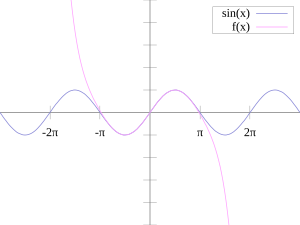 正弦函数(蓝色)十分接近于它的7次泰勒级数(粉色) 正弦函数(蓝色)十分接近于它的7次泰勒级数(粉色)
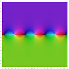
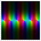
在几何学中,三角函数的定义建立在几何直观上,只用几何和极限的性质就可以直接得知正弦和餘弦的導數。在分析学中,三角函數是解析函數,数学家利用泰勒級數给出了不依赖几何直观的代数定义[11]: sin x = ∑ n = 0 ∞ ( − 1 ) n x 2 n + 1 ( 2 n + 1 ) ! = x − x 3 3 ! + x 5 5 ! − x 7 7 ! + ⋯ {\displaystyle \sin x=\sum _{n=0}^{\infty }{\frac {(-1)^{n}x^{2n+1}}{(2n+1)!}}=x-{\frac {x^{3}}{3!}}+{\frac {x^{5}}{5!}}-{\frac {x^{7}}{7!}}+\cdots } cos x = ∑ n = 0 ∞ ( − 1 ) n x 2 n ( 2 n ) ! = 1 − x 2 2 ! + x 4 4 ! − x 6 6 ! + ⋯ {\displaystyle \cos x=\sum _{n=0}^{\infty }{\frac {(-1)^{n}x^{2n}}{(2n)!}}=1-{\frac {x^{2}}{2!}}+{\frac {x^{4}}{4!}}-{\frac {x^{6}}{6!}}+\cdots }可以证明以上的无穷级数对任意实数 x {\displaystyle x} 都是收敛的,所以很好地定义了正弦和余弦函数。 三角函数的级数定义經常用作严格处理三角函数和起点应用(比如,在傅立叶级数中),因为无穷级数的理论可以从实数系的基础发展而来,不需要任何几何方面的考虑。这样,这些函数的可微性和连续性便可以单独从级数定义来确立。 其他三角函数的级数定义:[12] tan x = ∑ n = 1 ∞ ( − 1 ) n − 1 2 2 n ( 2 2 n − 1 ) B 2 n x 2 n − 1 ( 2 n ) ! = x + x 3 3 + 2 x 5 15 + 17 x 7 315 + ⋯ ( | x | x = ∑ n = 0 ∞ ( − 1 ) n + 1 2 ( 2 2 n − 1 − 1 ) B 2 n x 2 n − 1 ( 2 n ) ! = 1 x + x 6 + 7 x 3 360 + 31 x 5 15120 + ⋯ ( 0 x = ∑ n = 0 ∞ ( − 1 ) n E n x 2 n ( 2 n ) ! = 1 + x 2 2 + 5 x 4 24 + 61 x 6 720 + ⋯ ( | x | x = ∑ n = 0 ∞ ( − 1 ) n 2 2 n B 2 n x 2 n − 1 ( 2 n ) ! = 1 x − x 3 − x 3 45 − 2 x 5 945 − ⋯ ( 0 = cos θ + i sin θ {\displaystyle e^{{\mathrm {i} }\theta }=\cos \theta +{\mathrm {i} }\sin \theta \,} 。(i是虚数单位)欧拉首先注意到这关系式,因此叫做欧拉公式[13]。从中可推出,对实数x, cos x = Re ( e i x ) , sin x = Im ( e i x ) {\displaystyle \cos x\,=\,\operatorname {Re} \;\left(e^{{\mathrm {i} }x}\right)\;\;,\qquad \quad \sin x\,=\,\operatorname {Im} \;\left(e^{{\mathrm {i} }x}\right)}进一步还可定义对複自变量z的三角函数: sin z = ∑ n = 0 ∞ ( − 1 ) n ( 2 n + 1 ) ! z 2 n + 1 = e i z − e − i z 2 i = − i sinh ( i z ) {\displaystyle \sin z\,=\,\sum _{n=0}^{\infty }{\frac {(-1)^{n}}{(2n+1)!}}z^{2n+1}\,=\,{e^{{\mathrm {i} }z}-e^{-{\mathrm {i} }z} \over 2{\mathrm {i} }}=-{\mathrm {i} }\sinh \left({\mathrm {i} }z\right)} cos z = ∑ n = 0 ∞ ( − 1 ) n ( 2 n ) ! z 2 n = e i z + e − i z 2 = cosh ( i z ) {\displaystyle \cos z\,=\,\sum _{n=0}^{\infty }{\frac {(-1)^{n}}{(2n)!}}z^{2n}\,=\,{e^{{\mathrm {i} }z}+e^{-{\mathrm {i} }z} \over 2}=\cosh \left({\mathrm {i} }z\right)} sin ( a + b i ) = sin a cosh b + ( cos a sinh b ) i {\displaystyle \sin(a+b\mathrm {i} )=\sin a\cosh b+(\cos a\sinh b)\mathrm {i} } cos ( a + b i ) = cos a cosh b − ( sin a sinh b ) i {\displaystyle \cos(a+b\mathrm {i} )=\cos a\cosh b-(\sin a\sinh b)\mathrm {i} } tan ( a + b i ) = tan a + ( tanh b ) i 1 − ( tan a tanh b ) i {\displaystyle \tan(a+b\mathrm {i} )={\frac {\tan a+(\tanh b)\mathrm {i} }{1-(\tan a\tanh b)\mathrm {i} }}}(其中 sinh {\displaystyle \sinh } 、 cosh {\displaystyle \cosh } 、 tanh {\displaystyle \tanh } 為雙曲函數,其馬勞克林級數與對應的三角函數很類似,只差在正負號) 複平面中的三角函數(亮度表示函數值的絕對值,色相表示函數值的主輻角)


 sin
(
z
)
{\displaystyle \sin(z)}
cos
(
z
)
{\displaystyle \cos(z)}
tan
(
z
)
{\displaystyle \tan(z)}
cot
(
z
)
{\displaystyle \cot(z)}
sec
(
z
)
{\displaystyle \sec(z)}
csc
(
z
)
{\displaystyle \csc(z)}
较少見的三角函數[编辑]
sin
(
z
)
{\displaystyle \sin(z)}
cos
(
z
)
{\displaystyle \cos(z)}
tan
(
z
)
{\displaystyle \tan(z)}
cot
(
z
)
{\displaystyle \cot(z)}
sec
(
z
)
{\displaystyle \sec(z)}
csc
(
z
)
{\displaystyle \csc(z)}
较少見的三角函數[编辑]
 單位圓的三角函數,包括了兩種正矢(versin、vercos)、餘矢(coversin、covercos)、外正割和外餘割 單位圓的三角函數,包括了兩種正矢(versin、vercos)、餘矢(coversin、covercos)、外正割和外餘割
除了上述六種基本函數,史上還有下列幾種较少見的三角函数: 正矢 v e r s i n θ = 1 − cos θ {\displaystyle \mathrm {versin} \;\theta =1-\cos \theta } 半正矢 h a v e r s i n θ = 1 − cos θ 2 {\displaystyle \mathrm {haversin} \;\theta ={\frac {1-\cos \theta }{2}}} v e r c o s i n θ = 1 + cos θ {\displaystyle \mathrm {vercosin} \;\theta =1+\cos \theta } h a v e r c o s i n θ = 1 + cos θ 2 {\displaystyle \mathrm {havercosin} \;\theta ={\frac {1+\cos \theta }{2}}} 餘矢 c o v e r s i n θ = 1 − sin θ {\displaystyle \mathrm {coversin} \;\theta =1-\sin \theta } 半餘矢 h a c o v e r s i n θ = 1 − sin θ 2 {\displaystyle \mathrm {hacoversin} \;\theta ={\frac {1-\sin \theta }{2}}} c o v e r c o s i n θ = 1 + sin θ {\displaystyle \mathrm {covercosin} \;\theta =1+\sin \theta } h a c o v e r c o s i n θ = 1 + sin θ 2 {\displaystyle \mathrm {hacovercosin} \;\theta ={\frac {1+\sin \theta }{2}}} 外正割 e x s e c θ = sec θ − 1 {\displaystyle \mathrm {exsec} \;\theta =\sec \theta -1} 外餘割 e x c s c θ = csc θ − 1 {\displaystyle \mathrm {excsc} \;\theta =\csc \theta -1} 微分方程定义[编辑]三角函数在物理学是研究振动和波不可或缺的工具,如简谐振动满足以下微分方程,正弦和余弦函数都满足 y ″ + y = 0 {\displaystyle y''+y=0\,}就是说,它们加上自己的二阶导数都等于0函数。在由所有这條方程的解的二维向量空间 V {\displaystyle V} 中,正弦函数是满足初始条件 y ( 0 ) = 0 {\displaystyle y(0)=0} 和 y ′ ( 0 ) = 1 {\displaystyle y'(0)=1} 的唯一解,而余弦函数是满足初始条件 y ( 0 ) = 1 {\displaystyle y(0)=1} 和 y ′ ( 0 ) = 0 {\displaystyle y'(0)=0} 的唯一解[14]。因为正弦和余弦函数是线性无关的,它们在一起形成了 V {\displaystyle V} 的基。这种定义正弦和余弦函数的方法本质上等价于使用欧拉公式。(参见线性微分方程)。很明显这條微分方程不只用来定义正弦和余弦函数,还可用来证明正弦和余弦函数的三角恒等式。进一步的,观察到正弦和余弦函数满足 y ″ = − y {\displaystyle y''=-y\,} ,这意味着它们是二阶导数算子的特征函数。 正切函数是非线性微分方程 y ′ = 1 + y 2 {\displaystyle y'=1+y^{2}\,}满足初始条件 y ( 0 ) = 0 {\textstyle y(0)=0} 的唯一解。有个非常有趣的形象证明证明了正切函数满足这微分方程,参见Needham的Visual Complex Analysis。[15] 弧度的重要性[编辑]弧度通过测量沿着单位圆的路径的长度而指定一角,并构成正弦和余弦函数的特定辐角。特别是,只有映射弧度到比率的那些正弦和余弦函数才满足描述它们的经典微分方程。如果正弦和余弦函数的弧度辐角是正比于频率的 f ( x ) = sin ( k x ) ; k ≠ 0 , k ≠ 1 {\displaystyle f(x)=\sin(kx);k\neq 0,k\neq 1\,}则导数将正比于“振幅”。 f ′ ( x ) = k cos ( k x ) {\displaystyle f'(x)=k\cos(kx)\,} 。这里的 k {\displaystyle k} 是表示在单位之间映射的常数。如果 x {\displaystyle x} 是度,则 k = π 180 ∘ {\displaystyle k={\frac {\pi }{180^{\circ }}}} 。如果 x {\displaystyle x} 是圈(轉, 2 π {\displaystyle 2\pi } 弧度, 360 {\displaystyle 360} 度),則 k = 2 π {\displaystyle k=2\pi }这意味着使用度(或圈)的正弦的二阶导数不满足微分方程 y ″ = − y {\displaystyle y''=-y\,} ,但满足 y ″ = − k 2 y {\displaystyle y''=-k^{2}y\,} ;对余弦也是类似的。 这意味着这些正弦和余弦是不同的函数,因此只有它的辐角是弧度的条件下,正弦的四阶导数才再次是正弦。因为凡是作为函数意义上的正弦、余弦、正切,都只用弧度定义,而不用360度的角度定义。 利用函数方程定义三角函数[编辑]在数学分析中,可以利用基于和差公式这样的性质的函数方程来定义三角函数。例如,取用给定此种公式和毕达哥拉斯恒等式,可以证明只有两个实函数满足这些条件。即存在唯一的一对实函数 sin {\displaystyle \sin } 和 cos {\displaystyle \cos } 使得对于所有实数 x {\displaystyle x} 和 y {\displaystyle y} ,下列方程成立[16]: sin 2 x + cos 2 x = 1 , {\displaystyle \sin ^{2}\!x+\cos ^{2}\!x=1,\,} sin ( x + y ) = sin x cos y + cos x sin y , {\displaystyle \sin(x+y)=\sin \!x\cos \!y+\cos \!x\sin \!y,\,} cos ( x + y ) = cos x cos y − sin x sin y , {\displaystyle \cos(x+y)=\cos \!x\cos \!y-\sin \!x\sin \!y,\,}并满足附加条件 0 π 2 = 1 {\displaystyle \sin {\frac {\pi }{2}}=1} )开始并重复应用半角和和差公式而生成[17]。现代计算机使用了各种技术。[18]一个常见的方式,特别是在有浮点单元的高端处理器上,是组合多项式或有理式逼近(比如切比雪夫逼近、最佳一致逼近和Padé逼近,和典型用于更高或可变精度的泰勒级数和罗朗级数)和范围简约与表查找—首先在一个较小的表中查找最接近的角度,然后使用多项式来计算修正。[19]在缺乏硬件乘法器的简单设备上,有叫做CORDIC算法的一个更有效算法(和相关技术),因为它只用了移位和加法。出于性能的原因,所有这些方法通常都用硬件来实现。 对于非常高精度的运算,在级数展开收敛变得太慢的时候,可以用算术几何平均来逼近三角函数,它自身通过复数椭圆积分来逼近三角函数。[20] 三角函数的特殊值[编辑] 主条目:三角函数精确值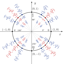 大小为
30
∘
{\displaystyle 30^{\circ }}
和
45
∘
{\displaystyle 45^{\circ }}
的整数倍的
θ
{\displaystyle \theta }
角和它们的精确正弦和余弦值标注在单位圆上。
θ
{\displaystyle \theta }
角均用弧度制和角度制表示。
θ
{\displaystyle \theta }
角所对应的单位圆上的点的坐标为(
cos
θ
{\displaystyle \cos \theta }
,
sin
θ
{\displaystyle \sin \theta }
) 大小为
30
∘
{\displaystyle 30^{\circ }}
和
45
∘
{\displaystyle 45^{\circ }}
的整数倍的
θ
{\displaystyle \theta }
角和它们的精确正弦和余弦值标注在单位圆上。
θ
{\displaystyle \theta }
角均用弧度制和角度制表示。
θ
{\displaystyle \theta }
角所对应的单位圆上的点的坐标为(
cos
θ
{\displaystyle \cos \theta }
,
sin
θ
{\displaystyle \sin \theta }
)
特殊角度可用勾股定理(即毕氏定理)人手輕易计出三角函数的值。 π / 60 {\displaystyle \pi /60} 弧度(3°)的任何整数倍之正弦、余弦和正切都可人手计算。以下是常用的特殊函数值[21]。 函数 0 ( 0 ∘ ) {\displaystyle 0\ (0^{\circ })} π 12 ( 15 ∘ ) {\displaystyle {\frac {\pi }{12}}\ (15^{\circ })} π 6 ( 30 ∘ ) {\displaystyle {\frac {\pi }{6}}\ (30^{\circ })} π 4 ( 45 ∘ ) {\displaystyle {\frac {\pi }{4}}\ (45^{\circ })} π 3 ( 60 ∘ ) {\displaystyle {\frac {\pi }{3}}\ (60^{\circ })} 5 π 12 ( 75 ∘ ) {\displaystyle {\frac {5\pi }{12}}\ (75^{\circ })} π 2 ( 90 ∘ ) {\displaystyle {\frac {\pi }{2}}\ (90^{\circ })} sin {\displaystyle \sin } 0 {\displaystyle 0} 6 − 2 4 {\displaystyle {\frac {{\sqrt {6}}-{\sqrt {2}}}{4}}} 1 2 {\displaystyle {\frac {1}{2}}} 2 2 {\displaystyle {\frac {\sqrt {2}}{2}}} 3 2 {\displaystyle {\frac {\sqrt {3}}{2}}} 6 + 2 4 {\displaystyle {\frac {{\sqrt {6}}+{\sqrt {2}}}{4}}} 1 {\displaystyle 1} cos {\displaystyle \cos } 1 {\displaystyle 1} 6 + 2 4 {\displaystyle {\frac {{\sqrt {6}}+{\sqrt {2}}}{4}}} 3 2 {\displaystyle {\frac {\sqrt {3}}{2}}} 2 2 {\displaystyle {\frac {\sqrt {2}}{2}}} 1 2 {\displaystyle {\frac {1}{2}}} 6 − 2 4 {\displaystyle {\frac {{\sqrt {6}}-{\sqrt {2}}}{4}}} 0 {\displaystyle 0} tan {\displaystyle \tan } 0 {\displaystyle 0} 2 − 3 {\displaystyle 2-{\sqrt {3}}} 3 3 {\displaystyle {\frac {\sqrt {3}}{3}}} 1 {\displaystyle 1} 3 {\displaystyle {\sqrt {3}}} 2 + 3 {\displaystyle 2+{\sqrt {3}}} ± ∞ {\displaystyle \pm \infty } cot {\displaystyle \cot } ± ∞ {\displaystyle \pm \infty } 2 + 3 {\displaystyle 2+{\sqrt {3}}} 3 {\displaystyle {\sqrt {3}}} 1 {\displaystyle 1} 3 3 {\displaystyle {\frac {\sqrt {3}}{3}}} 2 − 3 {\displaystyle 2-{\sqrt {3}}} 0 {\displaystyle 0} sec {\displaystyle \sec } 1 {\displaystyle 1} 6 − 2 {\displaystyle {\sqrt {6}}-{\sqrt {2}}} 2 3 3 {\displaystyle {\frac {2{\sqrt {3}}}{3}}} 2 {\displaystyle {\sqrt {2}}} 2 {\displaystyle 2} 6 + 2 {\displaystyle {\sqrt {6}}+{\sqrt {2}}} ± ∞ {\displaystyle \pm \infty } csc {\displaystyle \csc } ± ∞ {\displaystyle \pm \infty } 6 + 2 {\displaystyle {\sqrt {6}}+{\sqrt {2}}} 2 {\displaystyle 2} 2 {\displaystyle {\sqrt {2}}} 2 3 3 {\displaystyle {\frac {2{\sqrt {3}}}{3}}} 6 − 2 {\displaystyle {\sqrt {6}}-{\sqrt {2}}} 1 {\displaystyle 1}注: ± ∞ {\displaystyle \pm \infty } 有时会写作无定义(不存在)。 反三角函数[编辑] 主条目:反三角函数三角函数属周期函数而不是单射函数,严格来说并没有反函数,要定义其反函数必须先限制三角函数的定义域,使得三角函数成为双射函数。基本的反三角函数定义为[9]: 反三角函数 定义 值域 arcsin ( x ) = y {\displaystyle \arcsin(x)=y\,} sin ( y ) = x {\displaystyle \sin(y)=x\,} − π 2 ≤ y ≤ π 2 {\displaystyle -{\frac {\pi }{2}}\leq y\leq {\frac {\pi }{2}}\,} arccos ( x ) = y {\displaystyle \arccos(x)=y\,} cos ( y ) = x {\displaystyle \cos(y)=x\,} 0 ≤ y ≤ π {\displaystyle 0\leq y\leq \pi \,} arctan ( x ) = y {\displaystyle \arctan(x)=y\,} tan ( y ) = x {\displaystyle \tan(y)=x\,} − π 2 ( x ) = y {\displaystyle \operatorname {arccsc}(x)=y\,} csc ( y ) = x {\displaystyle \csc(y)=x\,} − π 2 ≤ y ≤ π 2 , y ≠ 0 {\displaystyle -{\frac {\pi }{2}}\leq y\leq {\frac {\pi }{2}},y\neq 0\,} arcsec ( x ) = y {\displaystyle \operatorname {arcsec}(x)=y\,} sec ( y ) = x {\displaystyle \sec(y)=x\,} 0 ≤ y ≤ π , y ≠ π 2 {\displaystyle 0\leq y\leq \pi ,y\neq {\frac {\pi }{2}}\,} arccot ( x ) = y {\displaystyle \operatorname {arccot}(x)=y\,} cot ( y ) = x {\displaystyle \cot(y)=x\,} 0 1 {\displaystyle \sin ^{-1}} 和 cos − 1 {\displaystyle \cos ^{-1}} 经常用于 arcsin {\displaystyle \arcsin } 和 arccos {\displaystyle \arccos } 。使用这种符号的时候,反函数可能跟三角函数的倒数混淆。“ a r c {\displaystyle \mathrm {arc} } ”前缀可避免这种混淆,尽管“ arcsec {\displaystyle \operatorname {arcsec} } ”可能偶尔跟“arcsecond”混淆。正如正弦和余弦那样,反三角函数也可以根据无穷级数来定义。例如, arcsin z = z + ( 1 2 ) z 3 3 + ( 1 ⋅ 3 2 ⋅ 4 ) z 5 5 + ( 1 ⋅ 3 ⋅ 5 2 ⋅ 4 ⋅ 6 ) z 7 7 + ⋯ {\displaystyle \arcsin z=z+\left({\frac {1}{2}}\right){\frac {z^{3}}{3}}+\left({\frac {1\cdot 3}{2\cdot 4}}\right){\frac {z^{5}}{5}}+\left({\frac {1\cdot 3\cdot 5}{2\cdot 4\cdot 6}}\right){\frac {z^{7}}{7}}+\cdots }这些函数也可以通过证明它们是其他函数的原函数来定义。例如反正弦函数,可以写为如下积分[22]: arcsin ( x ) = ∫ 0 x 1 1 − z 2 d z , | x | i ln ( i z + 1 − z 2 ) {\displaystyle \arcsin(z)=-{\mathrm {i} }\ln \left({\mathrm {i} }z+{\sqrt {1-z^{2}}}\right)} arccos ( z ) = − i ln ( z + z 2 − 1 ) {\displaystyle \arccos(z)=-{\mathrm {i} }\ln \left(z+{\sqrt {z^{2}-1}}\right)} arctan ( z ) = i 2 ln ( 1 − i z 1 + i z ) {\displaystyle \arctan(z)={\frac {\mathrm {i} }{2}}\ln \left({\frac {1-{\mathrm {i} }z}{1+{\mathrm {i} }z}}\right)} 相关定理[编辑]三角函数,正如其名,在三角学十分重要。三角学研究发现了许多利用三角函数来刻画三角形、圆形或多边形的定理。 正弦定理[编辑] 主条目:正弦定理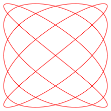 利萨茹(Lissajous)曲线,一种三角基的函数形成的图像 利萨茹(Lissajous)曲线,一种三角基的函数形成的图像
正弦定理声称对于边长为 a {\displaystyle a} 、 b {\displaystyle b} 和 c {\displaystyle c} 而相应角为 A {\displaystyle A} 、 B {\displaystyle B} 和 C {\displaystyle C} 的三角形,有[23]: a sin A = b sin B = c sin C = 2 R {\displaystyle {\frac {a}{\sin A}}={\frac {b}{\sin B}}={\frac {c}{\sin C}}=2R}其中 R {\displaystyle R} 是三角形的外接圆半径。正弦定理用于计算已知两角和一边时三角形的未知边长,是三角测量中常见情况,前述為數學常用。至於物理學應用為三分力且合力為0的情況。 余弦定理[编辑] 主条目:余弦定理余弦定理(也叫余弦公式)是托勒密定理的延伸[23]: c 2 = a 2 + b 2 − 2 a b cos C {\displaystyle c^{2}=a^{2}+b^{2}-2ab\cos C} 也可表示为 cos C = a 2 + b 2 − c 2 2 a b {\displaystyle \cos C={\frac {a^{2}+b^{2}-c^{2}}{2ab}}} 。 余弦定理用于确定三角形已知两边和一角时未知的值。 正切定理[24][编辑] 主条目:正切定理 a + b a − b = tan A + B 2 tan A − B 2 {\displaystyle {\frac {a+b}{a-b}}={\frac {\tan {\dfrac {A+B}{2}}}{\tan {\dfrac {A-B}{2}}}}} 餘切定理[编辑] 主条目:餘切定理cot α 2 = s − a ζ {\displaystyle \cot {\frac {\alpha }{2}}={\frac {s-a}{\zeta }}} 其中 ζ = 1 s ( s − a ) ( s − b ) ( s − c ) {\textstyle \zeta ={\sqrt {{\frac {1}{s}}(s-a)(s-b)(s-c)}}} 为三角形的内切圆半径, s = a + b + c 2 {\textstyle s={\frac {a+b+c}{2}}} 为三角形半周长。 周期函数[编辑] 谐波数目递增的方波的加法合成动画 谐波数目递增的方波的加法合成动画
三角函数在物理也重要,如用正弦和余弦函数描述简谐运动,它描述了很多自然现象,比如附着在弹簧上的物体的振动,挂在绳子上物体的小角度摆动。正弦和余弦函数是圆周运动的一维投影[25]。 三角函数在一般周期函数的研究中也很有用。这些函数有作为图像的特征波模式,在描述循环现象比如声波或光波的时候是很有用的。每个信号都可以记为不同频率的正弦和余弦函数的(通常无限)和[26];这是傅立叶分析的基础想法,这里的三角级数可以用来解微分方程的各种边值问题。例如,方波可以写为傅立叶级数[27] x s q u a r e ( t ) = 4 π ∑ k = 1 ∞ sin [ ( 2 k − 1 ) t ] ( 2 k − 1 ) {\displaystyle x_{\mathrm {square} }(t)={\frac {4}{\pi }}\sum _{k=1}^{\infty }{\sin {\left[(2k-1)t\right]} \over (2k-1)}} 。右边动画可見,只用幾项就形成非常准确的估计。 参见[编辑]正弦 · 餘弦 · 正切 · 餘切 · 正割 · 餘割  反函數 反函數
反正弦 · 反餘弦 · 反正切 · 反餘切 · 反正割 · 反餘割 其他函數正矢 · 餘矢 · cis函數 · 餘cis函數 · 半正矢 · 半餘矢 · 外正割 · 外餘割 · atan2 · 古德曼函數 雙曲函數雙曲正弦 · 雙曲餘弦 定理正弦定理 · 餘弦定理 · 正切定理 · 餘切定理 · 勾股定理 其他诱导公式 · 三角函數恆等式 · 三角函數精確值 · 三角函数积分表 · 三角函数表 · 雙曲三角函數 · 雙曲三角函數恆等式 规范控制
|
 )、余弦函数(
cos
{\displaystyle \cos }
)、余弦函数(
cos
{\displaystyle \cos }
 )和正切函数(
tan
{\displaystyle \tan }
)和正切函数(
tan
{\displaystyle \tan }
 或
tg
{\displaystyle \operatorname {tg} }
或
tg
{\displaystyle \operatorname {tg} }
 )[1];在航海学、测绘学和工程学等其他学科中还会用到例如余切函数(
cot
{\displaystyle \cot }
)[1];在航海学、测绘学和工程学等其他学科中还会用到例如余切函数(
cot
{\displaystyle \cot }
 或
ctg
{\displaystyle \operatorname {ctg} }
或
ctg
{\displaystyle \operatorname {ctg} }
 )、正割函数(
sec
{\displaystyle \sec }
)、正割函数(
sec
{\displaystyle \sec }
 )、余割函数(
csc
{\displaystyle \csc }
)、余割函数(
csc
{\displaystyle \csc }
 )、正矢函数和半正矢函数等其它三角函数。不同的三角函数之间的关系可以几何直观或计算得出,称为三角恒等式。
 可做出直角三角形,使一個内角為
θ
{\displaystyle \theta }
可做出直角三角形,使一個内角為
θ
{\displaystyle \theta }
 θ
{\displaystyle \theta }
θ
{\displaystyle \theta }
 θ
{\displaystyle \theta }
θ
{\displaystyle \theta }
 θ
{\displaystyle \theta }
θ
{\displaystyle \theta }
 θ
{\displaystyle \theta }
θ
{\displaystyle \theta }
 θ
{\displaystyle \theta }
θ
{\displaystyle \theta }
 以直角坐标系來定义[编辑]
 是平面直角坐标系
x
O
y
{\textstyle xOy}
是平面直角坐标系
x
O
y
{\textstyle xOy}
 中的一点,
θ
{\textstyle \theta }
中的一点,
θ
{\textstyle \theta }
 是横轴正向
O
x
→
{\textstyle {\vec {Ox}}}
是横轴正向
O
x
→
{\textstyle {\vec {Ox}}}
 逆时针旋转到
O
P
→
{\textstyle {\vec {OP}}}
逆时针旋转到
O
P
→
{\textstyle {\vec {OP}}}
 方向所形成的一個角,
r
=
x
2
+
y
2
>
0
{\textstyle r={\sqrt {x^{2}+y^{2}}}>0}
方向所形成的一個角,
r
=
x
2
+
y
2
>
0
{\textstyle r={\sqrt {x^{2}+y^{2}}}>0}
 是
P
{\textstyle P}
是
P
{\textstyle P}
 到原点
O
{\textstyle O}
到原点
O
{\textstyle O}
 的距离,则
θ
{\displaystyle \theta }
的距离,则
θ
{\displaystyle \theta }
 cos
θ
=
x
r
{\displaystyle \cos \theta ={\frac {x}{r}}}
cos
θ
=
x
r
{\displaystyle \cos \theta ={\frac {x}{r}}}
 tan
θ
=
y
x
{\displaystyle \tan \theta ={\frac {y}{x}}}
tan
θ
=
y
x
{\displaystyle \tan \theta ={\frac {y}{x}}}
 cot
θ
=
x
y
{\displaystyle \cot \theta ={\frac {x}{y}}}
cot
θ
=
x
y
{\displaystyle \cot \theta ={\frac {x}{y}}}
 sec
θ
=
r
x
{\displaystyle \sec \theta ={\frac {r}{x}}}
sec
θ
=
r
x
{\displaystyle \sec \theta ={\frac {r}{x}}}
 csc
θ
=
r
y
{\displaystyle \csc \theta ={\frac {r}{y}}}
csc
θ
=
r
y
{\displaystyle \csc \theta ={\frac {r}{y}}}

 ),那么三角函数就是取值为全体实数R,最小正周期(基本周期)为
2
π
{\displaystyle 2\pi }
),那么三角函数就是取值为全体实数R,最小正周期(基本周期)为
2
π
{\displaystyle 2\pi }
 cos
θ
=
cos
(
θ
+
2
π
k
)
,
∀
θ
∈
R
,
k
∈
Z
{\displaystyle \cos \theta =\cos \left(\theta +2\pi k\right),\quad \forall \theta \in \mathbb {R} ,\;\;k\in \mathbb {Z} }
cos
θ
=
cos
(
θ
+
2
π
k
)
,
∀
θ
∈
R
,
k
∈
Z
{\displaystyle \cos \theta =\cos \left(\theta +2\pi k\right),\quad \forall \theta \in \mathbb {R} ,\;\;k\in \mathbb {Z} }

 弧度或180°。
 中半径为1,以圆心为原点
O
{\displaystyle O}
中半径为1,以圆心为原点
O
{\displaystyle O}
 的单位圆来定义[1]。指定一角
θ
{\displaystyle \theta }
的单位圆来定义[1]。指定一角
θ
{\displaystyle \theta }
 为起始点,如果
θ
>
0
{\displaystyle \theta >0}
为起始点,如果
θ
>
0
{\displaystyle \theta >0}
 则将
O
A
{\displaystyle OA}
则将
O
A
{\displaystyle OA}
 以逆时针方向转动,如果
θ
θ
=
y
{\displaystyle \sin \theta =y}
以逆时针方向转动,如果
θ
θ
=
y
{\displaystyle \sin \theta =y}
 cos
θ
=
x
{\displaystyle \cos \theta =x}
cos
θ
=
x
{\displaystyle \cos \theta =x}
 tan
θ
=
y
x
{\displaystyle \tan \theta ={\frac {y}{x}}}
tan
θ
=
y
x
{\displaystyle \tan \theta ={\frac {y}{x}}}
 csc
θ
=
1
y
{\displaystyle \csc \theta ={\frac {1}{y}}}
csc
θ
=
1
y
{\displaystyle \csc \theta ={\frac {1}{y}}}
 基本性质[编辑]
 在直角坐标系平面上f(x)=sin(x)和f(x)=cos(x)函数的图像
 轴对称。正切函数和余切函数、正割函数和余割函数也分别如此。
 。
。
 。
1
+
cot
2
x
=
csc
2
x
{\displaystyle 1+\cot ^{2}\!x=\csc ^{2}\!x}
。
1
+
cot
2
x
=
csc
2
x
{\displaystyle 1+\cot ^{2}\!x=\csc ^{2}\!x}
 。
。
 cos
(
x
+
y
)
=
cos
x
cos
y
−
sin
x
sin
y
{\displaystyle \cos \left(x+y\right)=\cos x\cos y-\sin x\sin y}
cos
(
x
+
y
)
=
cos
x
cos
y
−
sin
x
sin
y
{\displaystyle \cos \left(x+y\right)=\cos x\cos y-\sin x\sin y}
 tan
(
x
+
y
)
=
tan
x
+
tan
y
1
−
tan
x
tan
y
{\displaystyle \tan \left(x+y\right)={\frac {\tan x+\tan y}{1-\tan x\tan y}}}
tan
(
x
+
y
)
=
tan
x
+
tan
y
1
−
tan
x
tan
y
{\displaystyle \tan \left(x+y\right)={\frac {\tan x+\tan y}{1-\tan x\tan y}}}

 cos
(
x
−
y
)
=
cos
x
cos
y
+
sin
x
sin
y
{\displaystyle \cos \left(x-y\right)=\cos x\cos y+\sin x\sin y}
cos
(
x
−
y
)
=
cos
x
cos
y
+
sin
x
sin
y
{\displaystyle \cos \left(x-y\right)=\cos x\cos y+\sin x\sin y}
 tan
(
x
−
y
)
=
tan
x
−
tan
y
1
+
tan
x
tan
y
{\displaystyle \tan \left(x-y\right)={\frac {\tan x-\tan y}{1+\tan x\tan y}}}
tan
(
x
−
y
)
=
tan
x
−
tan
y
1
+
tan
x
tan
y
{\displaystyle \tan \left(x-y\right)={\frac {\tan x-\tan y}{1+\tan x\tan y}}}

 cos
(
2
x
)
=
cos
2
x
−
sin
2
x
{\displaystyle \cos(2x)=\cos ^{2}x-\sin ^{2}x}
cos
(
2
x
)
=
cos
2
x
−
sin
2
x
{\displaystyle \cos(2x)=\cos ^{2}x-\sin ^{2}x}
 tan
(
2
x
)
=
2
tan
x
1
−
tan
2
x
{\displaystyle \tan(2x)={\frac {2\tan x}{1-\tan ^{2}x}}}
tan
(
2
x
)
=
2
tan
x
1
−
tan
2
x
{\displaystyle \tan(2x)={\frac {2\tan x}{1-\tan ^{2}x}}}

 cos
x
2
=
±
1
+
cos
x
2
{\displaystyle \cos {\frac {x}{2}}=\pm {\sqrt {\frac {1+\cos x}{2}}}}
cos
x
2
=
±
1
+
cos
x
2
{\displaystyle \cos {\frac {x}{2}}=\pm {\sqrt {\frac {1+\cos x}{2}}}}
 tan
x
2
=
±
1
−
cos
x
1
+
cos
x
=
1
−
cos
x
sin
x
=
sin
x
1
+
cos
x
{\displaystyle \tan {\frac {x}{2}}=\pm {\sqrt {\frac {1-\cos x}{1+\cos x}}}={\frac {1-\cos x}{\sin x}}={\frac {\sin x}{1+\cos x}}}
tan
x
2
=
±
1
−
cos
x
1
+
cos
x
=
1
−
cos
x
sin
x
=
sin
x
1
+
cos
x
{\displaystyle \tan {\frac {x}{2}}=\pm {\sqrt {\frac {1-\cos x}{1+\cos x}}}={\frac {1-\cos x}{\sin x}}={\frac {\sin x}{1+\cos x}}}
 微积分[编辑]
 cos
x
{\displaystyle \cos x}
cos
x
{\displaystyle \cos x}
 tan
x
{\displaystyle \tan x}
tan
x
{\displaystyle \tan x}
 cot
x
{\displaystyle \cot x}
cot
x
{\displaystyle \cot x}
 sec
x
{\displaystyle \sec x}
sec
x
{\displaystyle \sec x}
 csc
x
{\displaystyle \csc x}
csc
x
{\displaystyle \csc x}
 导数
cos
x
{\displaystyle \cos x}
导数
cos
x
{\displaystyle \cos x}
 sec
2
x
{\displaystyle \sec ^{2}x}
sec
2
x
{\displaystyle \sec ^{2}x}
 −
csc
2
x
{\displaystyle -\csc ^{2}x}
−
csc
2
x
{\displaystyle -\csc ^{2}x}
 sec
x
tan
x
{\displaystyle \sec {x}\tan {x}}
sec
x
tan
x
{\displaystyle \sec {x}\tan {x}}
 −
csc
x
cot
x
{\displaystyle -\csc {x}\cot {x}}
−
csc
x
cot
x
{\displaystyle -\csc {x}\cot {x}}
 反导数(不计常数项)
−
cos
x
{\displaystyle -\cos x}
反导数(不计常数项)
−
cos
x
{\displaystyle -\cos x}
 sin
x
{\displaystyle \sin x}
sin
x
{\displaystyle \sin x}
 ln
|
sin
x
|
{\displaystyle \ln \left|\sin x\right|}
ln
|
sin
x
|
{\displaystyle \ln \left|\sin x\right|}
 ln
|
sec
x
+
tan
x
|
{\displaystyle \ln \left|\sec x+\tan x\right|}
ln
|
sec
x
+
tan
x
|
{\displaystyle \ln \left|\sec x+\tan x\right|}
 ln
|
csc
x
−
cot
x
|
{\displaystyle \ln \left|\csc x-\cot x\right|}
ln
|
csc
x
−
cot
x
|
{\displaystyle \ln \left|\csc x-\cot x\right|}
 分析学定义[编辑]
級數定義[编辑]
分析学定义[编辑]
級數定義[编辑]
 cos
x
=
∑
n
=
0
∞
(
−
1
)
n
x
2
n
(
2
n
)
!
=
1
−
x
2
2
!
+
x
4
4
!
−
x
6
6
!
+
⋯
{\displaystyle \cos x=\sum _{n=0}^{\infty }{\frac {(-1)^{n}x^{2n}}{(2n)!}}=1-{\frac {x^{2}}{2!}}+{\frac {x^{4}}{4!}}-{\frac {x^{6}}{6!}}+\cdots }
cos
x
=
∑
n
=
0
∞
(
−
1
)
n
x
2
n
(
2
n
)
!
=
1
−
x
2
2
!
+
x
4
4
!
−
x
6
6
!
+
⋯
{\displaystyle \cos x=\sum _{n=0}^{\infty }{\frac {(-1)^{n}x^{2n}}{(2n)!}}=1-{\frac {x^{2}}{2!}}+{\frac {x^{4}}{4!}}-{\frac {x^{6}}{6!}}+\cdots }

 都是收敛的,所以很好地定义了正弦和余弦函数。
 。(i是虚数单位)

 cos
z
=
∑
n
=
0
∞
(
−
1
)
n
(
2
n
)
!
z
2
n
=
e
i
z
+
e
−
i
z
2
=
cosh
(
i
z
)
{\displaystyle \cos z\,=\,\sum _{n=0}^{\infty }{\frac {(-1)^{n}}{(2n)!}}z^{2n}\,=\,{e^{{\mathrm {i} }z}+e^{-{\mathrm {i} }z} \over 2}=\cosh \left({\mathrm {i} }z\right)}
cos
z
=
∑
n
=
0
∞
(
−
1
)
n
(
2
n
)
!
z
2
n
=
e
i
z
+
e
−
i
z
2
=
cosh
(
i
z
)
{\displaystyle \cos z\,=\,\sum _{n=0}^{\infty }{\frac {(-1)^{n}}{(2n)!}}z^{2n}\,=\,{e^{{\mathrm {i} }z}+e^{-{\mathrm {i} }z} \over 2}=\cosh \left({\mathrm {i} }z\right)}
 sin
(
a
+
b
i
)
=
sin
a
cosh
b
+
(
cos
a
sinh
b
)
i
{\displaystyle \sin(a+b\mathrm {i} )=\sin a\cosh b+(\cos a\sinh b)\mathrm {i} }
sin
(
a
+
b
i
)
=
sin
a
cosh
b
+
(
cos
a
sinh
b
)
i
{\displaystyle \sin(a+b\mathrm {i} )=\sin a\cosh b+(\cos a\sinh b)\mathrm {i} }
 cos
(
a
+
b
i
)
=
cos
a
cosh
b
−
(
sin
a
sinh
b
)
i
{\displaystyle \cos(a+b\mathrm {i} )=\cos a\cosh b-(\sin a\sinh b)\mathrm {i} }
cos
(
a
+
b
i
)
=
cos
a
cosh
b
−
(
sin
a
sinh
b
)
i
{\displaystyle \cos(a+b\mathrm {i} )=\cos a\cosh b-(\sin a\sinh b)\mathrm {i} }
 tan
(
a
+
b
i
)
=
tan
a
+
(
tanh
b
)
i
1
−
(
tan
a
tanh
b
)
i
{\displaystyle \tan(a+b\mathrm {i} )={\frac {\tan a+(\tanh b)\mathrm {i} }{1-(\tan a\tanh b)\mathrm {i} }}}
tan
(
a
+
b
i
)
=
tan
a
+
(
tanh
b
)
i
1
−
(
tan
a
tanh
b
)
i
{\displaystyle \tan(a+b\mathrm {i} )={\frac {\tan a+(\tanh b)\mathrm {i} }{1-(\tan a\tanh b)\mathrm {i} }}}

 、
cosh
{\displaystyle \cosh }
、
cosh
{\displaystyle \cosh }
 、
tanh
{\displaystyle \tanh }
、
tanh
{\displaystyle \tanh }
 為雙曲函數,其馬勞克林級數與對應的三角函數很類似,只差在正負號)
 cos
(
z
)
{\displaystyle \cos(z)}
cos
(
z
)
{\displaystyle \cos(z)}
 tan
(
z
)
{\displaystyle \tan(z)}
tan
(
z
)
{\displaystyle \tan(z)}
 cot
(
z
)
{\displaystyle \cot(z)}
cot
(
z
)
{\displaystyle \cot(z)}
 sec
(
z
)
{\displaystyle \sec(z)}
sec
(
z
)
{\displaystyle \sec(z)}
 csc
(
z
)
{\displaystyle \csc(z)}
csc
(
z
)
{\displaystyle \csc(z)}
 较少見的三角函數[编辑]
 半正矢
h
a
v
e
r
s
i
n
θ
=
1
−
cos
θ
2
{\displaystyle \mathrm {haversin} \;\theta ={\frac {1-\cos \theta }{2}}}
半正矢
h
a
v
e
r
s
i
n
θ
=
1
−
cos
θ
2
{\displaystyle \mathrm {haversin} \;\theta ={\frac {1-\cos \theta }{2}}}
 v
e
r
c
o
s
i
n
θ
=
1
+
cos
θ
{\displaystyle \mathrm {vercosin} \;\theta =1+\cos \theta }
v
e
r
c
o
s
i
n
θ
=
1
+
cos
θ
{\displaystyle \mathrm {vercosin} \;\theta =1+\cos \theta }
 h
a
v
e
r
c
o
s
i
n
θ
=
1
+
cos
θ
2
{\displaystyle \mathrm {havercosin} \;\theta ={\frac {1+\cos \theta }{2}}}
h
a
v
e
r
c
o
s
i
n
θ
=
1
+
cos
θ
2
{\displaystyle \mathrm {havercosin} \;\theta ={\frac {1+\cos \theta }{2}}}
 餘矢
c
o
v
e
r
s
i
n
θ
=
1
−
sin
θ
{\displaystyle \mathrm {coversin} \;\theta =1-\sin \theta }
餘矢
c
o
v
e
r
s
i
n
θ
=
1
−
sin
θ
{\displaystyle \mathrm {coversin} \;\theta =1-\sin \theta }
 半餘矢
h
a
c
o
v
e
r
s
i
n
θ
=
1
−
sin
θ
2
{\displaystyle \mathrm {hacoversin} \;\theta ={\frac {1-\sin \theta }{2}}}
半餘矢
h
a
c
o
v
e
r
s
i
n
θ
=
1
−
sin
θ
2
{\displaystyle \mathrm {hacoversin} \;\theta ={\frac {1-\sin \theta }{2}}}
 c
o
v
e
r
c
o
s
i
n
θ
=
1
+
sin
θ
{\displaystyle \mathrm {covercosin} \;\theta =1+\sin \theta }
c
o
v
e
r
c
o
s
i
n
θ
=
1
+
sin
θ
{\displaystyle \mathrm {covercosin} \;\theta =1+\sin \theta }
 h
a
c
o
v
e
r
c
o
s
i
n
θ
=
1
+
sin
θ
2
{\displaystyle \mathrm {hacovercosin} \;\theta ={\frac {1+\sin \theta }{2}}}
h
a
c
o
v
e
r
c
o
s
i
n
θ
=
1
+
sin
θ
2
{\displaystyle \mathrm {hacovercosin} \;\theta ={\frac {1+\sin \theta }{2}}}
 外正割
e
x
s
e
c
θ
=
sec
θ
−
1
{\displaystyle \mathrm {exsec} \;\theta =\sec \theta -1}
外正割
e
x
s
e
c
θ
=
sec
θ
−
1
{\displaystyle \mathrm {exsec} \;\theta =\sec \theta -1}
 外餘割
e
x
c
s
c
θ
=
csc
θ
−
1
{\displaystyle \mathrm {excsc} \;\theta =\csc \theta -1}
外餘割
e
x
c
s
c
θ
=
csc
θ
−
1
{\displaystyle \mathrm {excsc} \;\theta =\csc \theta -1}
 微分方程定义[编辑]

 中,正弦函数是满足初始条件
y
(
0
)
=
0
{\displaystyle y(0)=0}
中,正弦函数是满足初始条件
y
(
0
)
=
0
{\displaystyle y(0)=0}
 和
y
′
(
0
)
=
1
{\displaystyle y'(0)=1}
和
y
′
(
0
)
=
1
{\displaystyle y'(0)=1}
 的唯一解,而余弦函数是满足初始条件
y
(
0
)
=
1
{\displaystyle y(0)=1}
的唯一解,而余弦函数是满足初始条件
y
(
0
)
=
1
{\displaystyle y(0)=1}
 和
y
′
(
0
)
=
0
{\displaystyle y'(0)=0}
和
y
′
(
0
)
=
0
{\displaystyle y'(0)=0}
 的唯一解[14]。因为正弦和余弦函数是线性无关的,它们在一起形成了
V
{\displaystyle V}
的唯一解[14]。因为正弦和余弦函数是线性无关的,它们在一起形成了
V
{\displaystyle V}
 ,这意味着它们是二阶导数算子的特征函数。

 的唯一解。有个非常有趣的形象证明证明了正切函数满足这微分方程,参见Needham的Visual Complex Analysis。[15]

 。
。
 是表示在单位之间映射的常数。如果
x
{\displaystyle x}
是表示在单位之间映射的常数。如果
x
{\displaystyle x}
 。
。
 度),則
度),則

 ;
;
 ,下列方程成立[16]:
 sin
(
x
+
y
)
=
sin
x
cos
y
+
cos
x
sin
y
,
{\displaystyle \sin(x+y)=\sin \!x\cos \!y+\cos \!x\sin \!y,\,}
sin
(
x
+
y
)
=
sin
x
cos
y
+
cos
x
sin
y
,
{\displaystyle \sin(x+y)=\sin \!x\cos \!y+\cos \!x\sin \!y,\,}
 cos
(
x
+
y
)
=
cos
x
cos
y
−
sin
x
sin
y
,
{\displaystyle \cos(x+y)=\cos \!x\cos \!y-\sin \!x\sin \!y,\,}
cos
(
x
+
y
)
=
cos
x
cos
y
−
sin
x
sin
y
,
{\displaystyle \cos(x+y)=\cos \!x\cos \!y-\sin \!x\sin \!y,\,}

 )开始并重复应用半角和和差公式而生成[17]。
 和
45
∘
{\displaystyle 45^{\circ }}
和
45
∘
{\displaystyle 45^{\circ }}
 的整数倍的
θ
{\displaystyle \theta }
的整数倍的
θ
{\displaystyle \theta }
 ,
sin
θ
{\displaystyle \sin \theta }
,
sin
θ
{\displaystyle \sin \theta }
 )
)
 弧度(3°)的任何整数倍之正弦、余弦和正切都可人手计算。以下是常用的特殊函数值[21]。
 π
12
(
15
∘
)
{\displaystyle {\frac {\pi }{12}}\ (15^{\circ })}
π
12
(
15
∘
)
{\displaystyle {\frac {\pi }{12}}\ (15^{\circ })}
 π
6
(
30
∘
)
{\displaystyle {\frac {\pi }{6}}\ (30^{\circ })}
π
6
(
30
∘
)
{\displaystyle {\frac {\pi }{6}}\ (30^{\circ })}
 π
4
(
45
∘
)
{\displaystyle {\frac {\pi }{4}}\ (45^{\circ })}
π
4
(
45
∘
)
{\displaystyle {\frac {\pi }{4}}\ (45^{\circ })}
 π
3
(
60
∘
)
{\displaystyle {\frac {\pi }{3}}\ (60^{\circ })}
π
3
(
60
∘
)
{\displaystyle {\frac {\pi }{3}}\ (60^{\circ })}
 5
π
12
(
75
∘
)
{\displaystyle {\frac {5\pi }{12}}\ (75^{\circ })}
5
π
12
(
75
∘
)
{\displaystyle {\frac {5\pi }{12}}\ (75^{\circ })}
 π
2
(
90
∘
)
{\displaystyle {\frac {\pi }{2}}\ (90^{\circ })}
π
2
(
90
∘
)
{\displaystyle {\frac {\pi }{2}}\ (90^{\circ })}
 sin
{\displaystyle \sin }
sin
{\displaystyle \sin }
 6
−
2
4
{\displaystyle {\frac {{\sqrt {6}}-{\sqrt {2}}}{4}}}
6
−
2
4
{\displaystyle {\frac {{\sqrt {6}}-{\sqrt {2}}}{4}}}
 1
2
{\displaystyle {\frac {1}{2}}}
1
2
{\displaystyle {\frac {1}{2}}}
 2
2
{\displaystyle {\frac {\sqrt {2}}{2}}}
2
2
{\displaystyle {\frac {\sqrt {2}}{2}}}
 3
2
{\displaystyle {\frac {\sqrt {3}}{2}}}
3
2
{\displaystyle {\frac {\sqrt {3}}{2}}}
 6
+
2
4
{\displaystyle {\frac {{\sqrt {6}}+{\sqrt {2}}}{4}}}
6
+
2
4
{\displaystyle {\frac {{\sqrt {6}}+{\sqrt {2}}}{4}}}
 1
{\displaystyle 1}
1
{\displaystyle 1}
 cos
{\displaystyle \cos }
cos
{\displaystyle \cos }
 3
3
{\displaystyle {\frac {\sqrt {3}}{3}}}
3
3
{\displaystyle {\frac {\sqrt {3}}{3}}}
 1
{\displaystyle 1}
1
{\displaystyle 1}
 2
+
3
{\displaystyle 2+{\sqrt {3}}}
2
+
3
{\displaystyle 2+{\sqrt {3}}}
 ±
∞
{\displaystyle \pm \infty }
±
∞
{\displaystyle \pm \infty }
 cot
{\displaystyle \cot }
cot
{\displaystyle \cot }
 2
3
3
{\displaystyle {\frac {2{\sqrt {3}}}{3}}}
2
3
3
{\displaystyle {\frac {2{\sqrt {3}}}{3}}}
 2
{\displaystyle {\sqrt {2}}}
2
{\displaystyle {\sqrt {2}}}
 2
{\displaystyle 2}
2
{\displaystyle 2}
 6
+
2
{\displaystyle {\sqrt {6}}+{\sqrt {2}}}
6
+
2
{\displaystyle {\sqrt {6}}+{\sqrt {2}}}
 ±
∞
{\displaystyle \pm \infty }
±
∞
{\displaystyle \pm \infty }
 sin
(
y
)
=
x
{\displaystyle \sin(y)=x\,}
sin
(
y
)
=
x
{\displaystyle \sin(y)=x\,}
 −
π
2
≤
y
≤
π
2
{\displaystyle -{\frac {\pi }{2}}\leq y\leq {\frac {\pi }{2}}\,}
−
π
2
≤
y
≤
π
2
{\displaystyle -{\frac {\pi }{2}}\leq y\leq {\frac {\pi }{2}}\,}
 arccos
(
x
)
=
y
{\displaystyle \arccos(x)=y\,}
arccos
(
x
)
=
y
{\displaystyle \arccos(x)=y\,}
 cos
(
y
)
=
x
{\displaystyle \cos(y)=x\,}
cos
(
y
)
=
x
{\displaystyle \cos(y)=x\,}
 0
≤
y
≤
π
{\displaystyle 0\leq y\leq \pi \,}
0
≤
y
≤
π
{\displaystyle 0\leq y\leq \pi \,}
 arctan
(
x
)
=
y
{\displaystyle \arctan(x)=y\,}
arctan
(
x
)
=
y
{\displaystyle \arctan(x)=y\,}
 tan
(
y
)
=
x
{\displaystyle \tan(y)=x\,}
tan
(
y
)
=
x
{\displaystyle \tan(y)=x\,}
 −
π
2
(
x
)
=
y
{\displaystyle \operatorname {arccsc}(x)=y\,}
−
π
2
(
x
)
=
y
{\displaystyle \operatorname {arccsc}(x)=y\,}
 csc
(
y
)
=
x
{\displaystyle \csc(y)=x\,}
csc
(
y
)
=
x
{\displaystyle \csc(y)=x\,}
 −
π
2
≤
y
≤
π
2
,
y
≠
0
{\displaystyle -{\frac {\pi }{2}}\leq y\leq {\frac {\pi }{2}},y\neq 0\,}
−
π
2
≤
y
≤
π
2
,
y
≠
0
{\displaystyle -{\frac {\pi }{2}}\leq y\leq {\frac {\pi }{2}},y\neq 0\,}
 arcsec
(
x
)
=
y
{\displaystyle \operatorname {arcsec}(x)=y\,}
arcsec
(
x
)
=
y
{\displaystyle \operatorname {arcsec}(x)=y\,}
 sec
(
y
)
=
x
{\displaystyle \sec(y)=x\,}
sec
(
y
)
=
x
{\displaystyle \sec(y)=x\,}
 0
≤
y
≤
π
,
y
≠
π
2
{\displaystyle 0\leq y\leq \pi ,y\neq {\frac {\pi }{2}}\,}
0
≤
y
≤
π
,
y
≠
π
2
{\displaystyle 0\leq y\leq \pi ,y\neq {\frac {\pi }{2}}\,}
 arccot
(
x
)
=
y
{\displaystyle \operatorname {arccot}(x)=y\,}
arccot
(
x
)
=
y
{\displaystyle \operatorname {arccot}(x)=y\,}
 cot
(
y
)
=
x
{\displaystyle \cot(y)=x\,}
cot
(
y
)
=
x
{\displaystyle \cot(y)=x\,}
 0
1
{\displaystyle \sin ^{-1}}
0
1
{\displaystyle \sin ^{-1}}
 和
cos
−
1
{\displaystyle \cos ^{-1}}
和
cos
−
1
{\displaystyle \cos ^{-1}}
 经常用于
arcsin
{\displaystyle \arcsin }
经常用于
arcsin
{\displaystyle \arcsin }
 和
arccos
{\displaystyle \arccos }
和
arccos
{\displaystyle \arccos }
 。使用这种符号的时候,反函数可能跟三角函数的倒数混淆。“
a
r
c
{\displaystyle \mathrm {arc} }
。使用这种符号的时候,反函数可能跟三角函数的倒数混淆。“
a
r
c
{\displaystyle \mathrm {arc} }
 ”前缀可避免这种混淆,尽管“
arcsec
{\displaystyle \operatorname {arcsec} }
”前缀可避免这种混淆,尽管“
arcsec
{\displaystyle \operatorname {arcsec} }
 ”可能偶尔跟“arcsecond”混淆。

 arccos
(
z
)
=
−
i
ln
(
z
+
z
2
−
1
)
{\displaystyle \arccos(z)=-{\mathrm {i} }\ln \left(z+{\sqrt {z^{2}-1}}\right)}
arccos
(
z
)
=
−
i
ln
(
z
+
z
2
−
1
)
{\displaystyle \arccos(z)=-{\mathrm {i} }\ln \left(z+{\sqrt {z^{2}-1}}\right)}
 arctan
(
z
)
=
i
2
ln
(
1
−
i
z
1
+
i
z
)
{\displaystyle \arctan(z)={\frac {\mathrm {i} }{2}}\ln \left({\frac {1-{\mathrm {i} }z}{1+{\mathrm {i} }z}}\right)}
arctan
(
z
)
=
i
2
ln
(
1
−
i
z
1
+
i
z
)
{\displaystyle \arctan(z)={\frac {\mathrm {i} }{2}}\ln \left({\frac {1-{\mathrm {i} }z}{1+{\mathrm {i} }z}}\right)}
 相关定理[编辑]
 、
b
{\displaystyle b}
、
b
{\displaystyle b}
 和
c
{\displaystyle c}
和
c
{\displaystyle c}
 而相应角为
A
{\displaystyle A}
而相应角为
A
{\displaystyle A}
 、
B
{\displaystyle B}
、
B
{\displaystyle B}
 和
C
{\displaystyle C}
和
C
{\displaystyle C}
 的三角形,有[23]:

 是三角形的外接圆半径。正弦定理用于计算已知两角和一边时三角形的未知边长,是三角测量中常见情况,前述為數學常用。至於物理學應用為三分力且合力為0的情況。

 。
。
 餘切定理[编辑]
主条目:餘切定理
餘切定理[编辑]
主条目:餘切定理

 为三角形的内切圆半径,
s
=
a
+
b
+
c
2
{\textstyle s={\frac {a+b+c}{2}}}
为三角形的内切圆半径,
s
=
a
+
b
+
c
2
{\textstyle s={\frac {a+b+c}{2}}}
 为三角形半周长。
![{\displaystyle x_{\mathrm {square} }(t)={\frac {4}{\pi }}\sum _{k=1}^{\infty }{\sin {\left[(2k-1)t\right]} \over (2k-1)}}](https://wikimedia.org/api/rest_v1/media/math/render/svg/128f4a35c3192ee89a749b0341e978c2a07e6a6c) 。
。
【本文地址】
今日新闻 |
推荐新闻 |