【Stata基础】第二章 简单线性回归模型 |
您所在的位置:网站首页 › 最简单的线性回归模型 › 【Stata基础】第二章 简单线性回归模型 |
【Stata基础】第二章 简单线性回归模型
文章目录
一、练习二、线性回归模型1. 初步探索2. 简单OLS回归(最小二乘法)
三、二次式模型四、对数线性模型五、指示变量回归六、练习
一、练习
列出价格大于6000的国产汽车的价格sysuse auto, clear
list price if price > 6000 & foreign == 0
给出1978年维修记录少于3次或产地为国外的汽车价格和重量的描述性统计信息sum price weight if (rep78 < 3 | foreign == 1)
本数据中有多少辆国产汽车价格大于6000?count if price > 6000 & foreign == 0
列出 price wei len mpg turn foreign 变量的均值,标准差,中位数,最大值,最小值(对于这种要求,将一系列统计量以一张表格的形式展现出来更合适)tabstat price wei len mpg turn foreign, stat(mean sd median max min)
按国产和非国产为标准分类对price wei 进行描述性统计by foreign : sum price wei
将数据按照价格进行升序和降序排列gsort price
gsort -price
删除1978年维修记录缺失的数据drop if rep78 == .
将字符型变量make转换成数值型变量cenmakeencode make, gen(cenmake)
将price 转化成字符型变量tostring price, replace
将price 转化成数值型变量destring price, replace
生成一个虚拟变量,其中价格大于6000为1,否则表示为0gen vari = 1 if price > 6000
replace vari = 0 if price 6000
给出price wei len mpg 相关系数矩阵pwcorr price wei len mpg
画出price wei len mpg 的相关系数矩阵散点图(graph是最需要掌握的画图命令)graph matrix price wei len mpg
画出price频率直方图histogram price, frequency
画出price和weight的散点图scatter price weight
给price 和weight散点图加上price和wei的拟合线twoway (scatter price weight) (lfit price weight)
二、线性回归模型
做一个简单的OLS回归,其中被解释变量为price,解释变量为weight foreign
1. 初步探索
cd D:\Stata_Projects //进入存储数据的工作目录
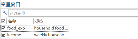
use "food.dta", clear //使用这个数据集
 * 得到数据之后,一般先浏览,检查数据,并看变量的描述性统计信息
* 画出food_exp与income的散点图,并保存
twoway (scatter food_exp income)
* 保存图片, 如果有了就替代
graph save food1, replace
* 一步到位
twoway (scatter food_exp income), saving(food1, replace)
* 得到数据之后,一般先浏览,检查数据,并看变量的描述性统计信息
* 画出food_exp与income的散点图,并保存
twoway (scatter food_exp income)
* 保存图片, 如果有了就替代
graph save food1, replace
* 一步到位
twoway (scatter food_exp income), saving(food1, replace)
 * 更丰富的画图功能, 使用help graph就可以查看到
twoway (scatter food_exp income) /// /* 基本语句,画什么的散点图 */
(lfit food_exp income), /// /*拟合线*/
ylabel(0(100)600) /// /* Y轴的刻度从0到600,间隔为100 */
xlabel(0(5)35) /// /* X轴刻度0-35,间隔5 */
title(食物消费数据) /// /* 图片名字 */
xtitle(每周收入) ///
ytitle(每周家庭食物花费)
* 还有更多的画图内容可以学习,图片的保存等也可以直接点击图片操作
* 更丰富的画图功能, 使用help graph就可以查看到
twoway (scatter food_exp income) /// /* 基本语句,画什么的散点图 */
(lfit food_exp income), /// /*拟合线*/
ylabel(0(100)600) /// /* Y轴的刻度从0到600,间隔为100 */
xlabel(0(5)35) /// /* X轴刻度0-35,间隔5 */
title(食物消费数据) /// /* 图片名字 */
xtitle(每周收入) ///
ytitle(每周家庭食物花费)
* 还有更多的画图内容可以学习,图片的保存等也可以直接点击图片操作

 2. 简单OLS回归(最小二乘法)
* food_ex = coef * income + ... 对income进行回归
regress food_exp income
2. 简单OLS回归(最小二乘法)
* food_ex = coef * income + ... 对income进行回归
regress food_exp income
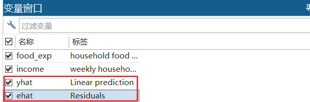
 * 计算y的拟合值,这里的y是food_exp'; xb是计算线性拟合值
predict yhat, xb //calculate linear prediction
* 计算残差项的拟合值
predict ehat, residuals
browse
* 计算y的拟合值,这里的y是food_exp'; xb是计算线性拟合值
predict yhat, xb //calculate linear prediction
* 计算残差项的拟合值
predict ehat, residuals
browse

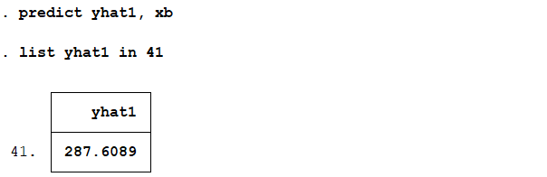
 * 做预测,预测其他的收入情况在该模型中的食物支出
* 例如,预测家庭每周收入2000$的家庭,每周食物支出
set obs 41 //本数据有40个观测值,我们多加一个观测值,但是没有定义具体观测值内容,它目前是缺失
replace income = 20 in 41 //将收入第41个观测值替换成20百
predict yhat1, xb
list yhat1 in 41
* 做预测,预测其他的收入情况在该模型中的食物支出
* 例如,预测家庭每周收入2000$的家庭,每周食物支出
set obs 41 //本数据有40个观测值,我们多加一个观测值,但是没有定义具体观测值内容,它目前是缺失
replace income = 20 in 41 //将收入第41个观测值替换成20百
predict yhat1, xb
list yhat1 in 41
 * 保存dta文件
* 直接点save菜单,或者输入下面命令
save "newfood.dta", replace
三、二次式模型
* 保存dta文件
* 直接点save菜单,或者输入下面命令
save "newfood.dta", replace
三、二次式模型
y = β 1 + β 2 ∗ x 2 + e y=\beta _1+ \beta_2*x^2 + e y=β1+β2∗x2+e * 二次式模型 use "br.dta",clear sum //sum, detail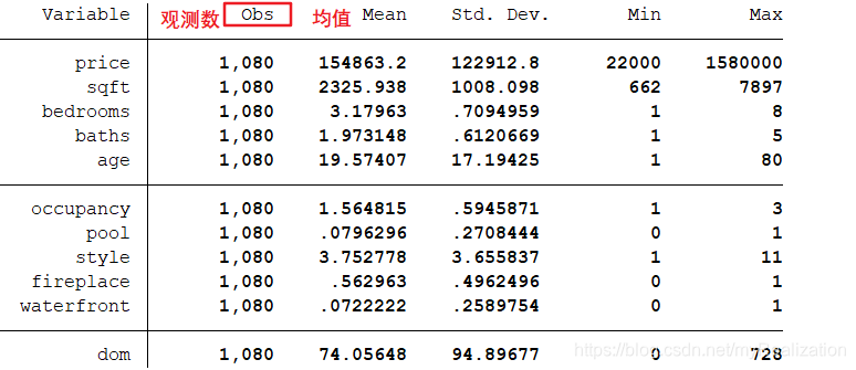 desc
desc
 gen sqft2 =sqft^2 //生成变量
regress price sqft2 //二次模型
predict priceq, xb
br price sqft sqft2 priceq
gen sqft2 =sqft^2 //生成变量
regress price sqft2 //二次模型
predict priceq, xb
br price sqft sqft2 priceq
 * 画出拟合曲线
twoway (scatter price sqft) /// /* 基本的点 */
(lfit price sqft, /// /* 拟合线 */
sort lwidth(medthick)) /*设定线的厚度 */
graph save br_quad1, replace //保存图片
twoway (scatter price sqft) /// /* 基本的点 */
(line price sqft, /// /* 折线 */
sort lwidth(medthick)) /*设定线的厚度 */
graph save br_quad2, replace //保存图片
twoway (scatter price sqft) /// /* 基本的点 */
(line priceq sqft, /// /* 折线 */
sort lwidth(medthick)) /*设定线的厚度 */
graph save br_quad3, replace //保存图片
graph combine "br_quad1" "br_quad2" "br_quad3"
* 比较三个图片区别
* 画出拟合曲线
twoway (scatter price sqft) /// /* 基本的点 */
(lfit price sqft, /// /* 拟合线 */
sort lwidth(medthick)) /*设定线的厚度 */
graph save br_quad1, replace //保存图片
twoway (scatter price sqft) /// /* 基本的点 */
(line price sqft, /// /* 折线 */
sort lwidth(medthick)) /*设定线的厚度 */
graph save br_quad2, replace //保存图片
twoway (scatter price sqft) /// /* 基本的点 */
(line priceq sqft, /// /* 折线 */
sort lwidth(medthick)) /*设定线的厚度 */
graph save br_quad3, replace //保存图片
graph combine "br_quad1" "br_quad2" "br_quad3"
* 比较三个图片区别
 四、对数线性模型
l n y = β 1 + β 2 x + e lny=\beta_1 + \beta_2x+e lny=β1+β2x+e histogram price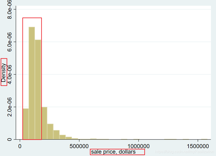 graph save price, replace
gen lnprice=ln(price) //price 存在一些值特别大,尾巴很长,为了把数据平滑一点,取对数
histogram lnprice,percent //更接近正态分布
graph save price, replace
gen lnprice=ln(price) //price 存在一些值特别大,尾巴很长,为了把数据平滑一点,取对数
histogram lnprice,percent //更接近正态分布
 reg lnprice sqft //对数线性模型回归
predict lpricef, xb //得到对数形式的拟合值
reg lnprice sqft //对数线性模型回归
predict lpricef, xb //得到对数形式的拟合值
 * 画出拟合曲线
generate pricef = exp(lpricef)
twoway (scatter price sqft)
(line pricef sqft, sort lwidth(medthick))
graph save br_loglin, replace
* 画出拟合曲线
generate pricef = exp(lpricef)
twoway (scatter price sqft)
(line pricef sqft, sort lwidth(medthick))
graph save br_loglin, replace
 五、指示变量回归
首先进一步学习创建虚拟变量/factor variables/指示变量: 方法1. 设定是否满足某个条件来生成,条件为真,取值 1 1 1,否则取 0 0 0: gen bh = (bedrooms>4) // 卧室数量大于四为大房子,取值为1 方法2. t a b u l a t e tabulate tabulate 创建指示变量。让每个可能的 b a t h s baths baths 取值都设定一个独立的虚拟变量: tabulate region, gen(reg) // Create indicator variables for region, called reg1, reg2, ... tabulate baths, gen(bath) // 为每个baths取值计数,gen(bath)就会产生5个指示变量bath1-5  六、练习
use "utown.dta", clear
describe //拿到数据的规定动作,了解数据内容和描述性统计信息
sum
六、练习
use "utown.dta", clear
describe //拿到数据的规定动作,了解数据内容和描述性统计信息
sum
 * 按照房子是否位于大学附近进行分类画图
histogram price if utown==0, width(12) start(130) percent ///
xtitle(House prices ($1000) in Golden Oaks) ///
xlabel(130(24)350) legend(off)
graph save utown_0, replace
* 按照房子是否位于大学附近进行分类画图
histogram price if utown==0, width(12) start(130) percent ///
xtitle(House prices ($1000) in Golden Oaks) ///
xlabel(130(24)350) legend(off)
graph save utown_0, replace
 histogram price if utown==1, width(12) start(130) percent ///
xtitle(House prices ($1000) in University Town) ///
xlabel(130(24)350) legend(off)
graph save utown_1, replace
graph combine "utown_0" "utown_1", col(1) iscale(1)
*把两张图放在一张图上,col(#)分成几列显示,iscale()文本和标记的大小
graph save combined ,replace
histogram price if utown==1, width(12) start(130) percent ///
xtitle(House prices ($1000) in University Town) ///
xlabel(130(24)350) legend(off)
graph save utown_1, replace
graph combine "utown_0" "utown_1", col(1) iscale(1)
*把两张图放在一张图上,col(#)分成几列显示,iscale()文本和标记的大小
graph save combined ,replace


histogram每一个语句的意思需要好好理解,例如: histogram price if utown==0:意思是做房屋不位于大学附近的房子的价格的直方图;width(12)是柱子宽度为 12 12 12 个刻度;start(130)价格从 130 130 130 开始画(price最小值为 134 134 134,这样x轴不会从 0 0 0 开始)percent表示纵轴为占比;xlabel表示 x x x 轴刻度从 130 130 130 到 350 350 350,单位刻度(即间隔刻度)为 25 25 25;legend(off)表示不显示图例 label define utownlabel 0 "Golden Oaks" 1 "University Town" //定义utown值的label label value utown utownlabel //将utown的label也按照值的label定义 label variable varname 给变量定标签label define labelname 给变量的值定义标签label value varlist(一列变量名) labelname 将取值的标签定义给变量 * by(utown, cols(1)) 按照utown分组画图 histogram price, by(utown, cols(2)) start(130) percent xtitle(House prices ($1000)) xlabel(130(24)350) legend(off) graph save combined2, replace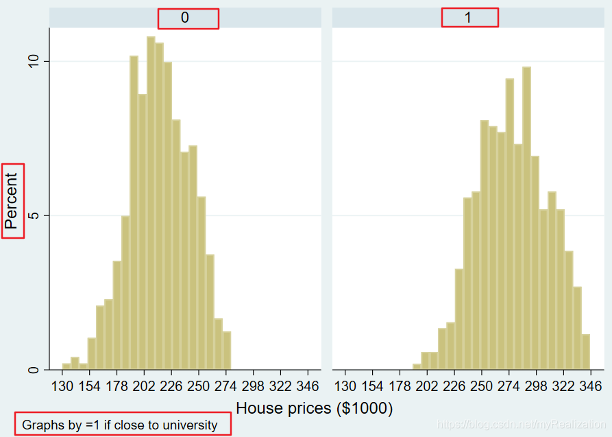 检验独立社区房价的描述性统计信息 sum price if utown == 0 sum price if utown == 1
  复习,用 bysort 分组统计 bysort utown:sum price 复习,用 bysort 分组统计 bysort utown:sum price  另一种写法 by utown,sort:sum price 另一种写法 by utown,sort:sum price 
b y by by and b y s o r t bysort bysort are really the same command; b y s o r t bysort bysort is just b y by by with the s o r t sort sort option. |
【本文地址】