|
数据集来源:https://scikit-learn.org/stable/modules/generated/sklearn.datasets.load_iris.html#sklearn.datasets.load_iris
1. 数据导入
鸢尾花数据可直接从Sklearn中的datasets 导出。sklearn.datasets.load_iris(*, return_X_y=False, as_frame=False) 该Iris中有两个属性,分别是:iris.data和iris.target
data里是一个矩阵,每一列代表了萼片或花瓣的长宽,一共4列,每一列代表某个被测量的鸢尾植物,一共采样了150条记录。target 代表花的种类return_X_y 指要不要返回 (data, target)两组值,如果选datasets.load_iris(return_X_y=True)即返回上面两组值,默认是Falseas_frame 如果用True,则返回DataFrame格式。 注:New in version 0.23. 0.23之前的版本没有这个,用help(sklearn)查看目前版本。
from sklearn import datasets
iris = datasets.load_iris() #鸢尾花数据可直接从Sklearn中的datasets 导出
iris #直接从datasets中读取,返回的是字典格式的数据
print(type(iris['data'])) #data数据类型
print(iris['data'].shape) #data结构
print(iris['target'].shape) #结构
print(iris['target_names']) #iris中的targetname
print(iris['target']) #iris中的target列
#切分成X和Y
X, y = iris.data, iris.target
#格式转换,整合成表格
iris_data = pd.DataFrame(np.hstack((X, y.reshape(-1, 1))),index = range(X.shape[0]),columns=['sepal_length_cm','sepal_width_cm','petal_length_cm','petal_width_cm','class'] )

2.了解数据
iris_data.info() #查看数据类型`
 再例行先来一个描述性分析: 再例行先来一个描述性分析:
iris_data.describe() #统计分析

#可视化分析,查看到不同特征之间的关系以及分布
sns.pairplot(iris_data.dropna(),hue = 'class’)

热力图: 分析特征之间的相关性
fig=plt.gcf()
fig.set_size_inches(12, 8)
fig=sns.heatmap(iris_data.corr(), annot=True, cmap='GnBu', linewidths=1, linecolor='k', square=True, mask=False, vmin=-1, vmax=1, cbar_kws={"orientation": "vertical"}, cbar=True)

3.数据集训练集切分
#数据集训练集切分
from sklearn.model_selection import train_test_split
X_train, X_test, y_train, y_test = train_test_split(X, y, test_size=0.2, random_state=20, shuffle=True)
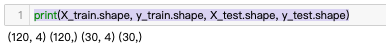
print(X_train.shape, y_train.shape, X_test.shape, y_test.shape)#结果可以看到把样本分成了120和30 两个样本
 再画个图看看具体三类花的分布: 再画个图看看具体三类花的分布:
参考链接:https://blog.csdn.net/Shine_rise/article/details/102975238
#数据可视化
plt.scatter(X_train[y_train == 0][:, 0], X_train[y_train == 0][:, 1], color='r')
plt.scatter(X_train[y_train == 1][:, 0], X_train[y_train == 1][:, 1], color='g')
plt.scatter(X_train[y_train == 2][:, 0], X_train[y_train == 2][:, 1], color='b')
plt.xlabel('sepal length')
plt.ylabel('sepal width')
plt.show()

4.建模
# Logistic Regression
model = LogisticRegression()
model.fit(X_train, y_train)
prediction = model.predict(X_test)
print('The accuracy of the Logistic Regression is {0}'.format(metrics.accuracy_score(prediction,y_test)))
# Support Vector Machine
model = svm.SVC()
model.fit(X_train, y_train)
prediction = model.predict(X_test)
print('The accuracy of the SVM is: {0}'.format(metrics.accuracy_score(prediction,y_test)))
# Decision Tree
model=DecisionTreeClassifier()
prediction = model.predict(X_test)
print('The accuracy of the Decision Tree is:{0}'.format(metrics.accuracy_score(prediction,y_test)))
# K-Nearest Neighbours
model=KNeighborsClassifier(n_neighbors=3)
model.fit(X_train, y_train)
prediction = model.predict(X_test)
print('The accuracy of the KNN is: {0}'.format(metrics.accuracy_score(prediction,y_test)))
结果SVM最好,其他都一样。 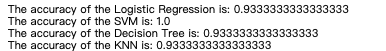
模型评估可视化
混淆矩阵(这里直接用了上面的X_test, y_test,即KNN的结果)
from sklearn.metrics import plot_confusion_matrix #导包
class_names = iris.target_names #用来命名的
np.set_printoptions(precision=2) #数组格式化打印(指定小数点位数)
# Plot non-normalized confusion matrix
titles_options = [("Confusion matrix, without normalization", None),
("Normalized confusion matrix", 'true')]
for title, normalize in titles_options:
disp = plot_confusion_matrix(model, X_test, y_test,
display_labels=class_names,
cmap=plt.cm.Blues,
normalize=normalize)
disp.ax_.set_title(title)
print(title)
print(disp.confusion_matrix)
plt.show()
结果输出: 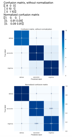 再画一下SVM,这里直接用了个整合的代码(建模+画图) 再画一下SVM,这里直接用了个整合的代码(建模+画图)
# Support Vector Machine
model = svm.SVC()
model.fit(X_train, y_train)
prediction = model.predict(X_test)
print('The accuracy of the SVM is: {0}'.format(metrics.accuracy_score(prediction,y_test)))
from sklearn.metrics import plot_confusion_matrix
class_names = iris.target_names #用来命名的
np.set_printoptions(precision=2) #数组格式化打印(指定小数点位数)
# Plot non-normalized confusion matrix
titles_options = [("Confusion matrix, without normalization", None),
("Normalized confusion matrix", 'true')]
for title, normalize in titles_options:
disp = plot_confusion_matrix(model, X_test, y_test,
display_labels=class_names,
cmap=plt.cm.Blues,
normalize=normalize)
disp.ax_.set_title(title)
print(title)
print(disp.confusion_matrix)
plt.show()
结果如下图,可见都是整整齐齐地排在对角线上,结论和之前的accuracy_score一样,SVM准确度要比KNN高 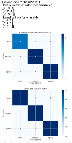
|