|
文章目录
运动模糊图像的复原简单的先退化后复原。复原拍摄的运动模糊图像
运动模糊图像的复原
看了网上很多方法,都是用退化函数将图像先遍模糊,然后再用同样的退化函数复原原图像。使用的大多是维纳滤波。那么能否将我们自己拍摄的运动模糊图像进行复原呢?小白菜尝试了很久,得到了一个效果还可以的结果,给大家分享一下。
下面给出我使用的退化函数: 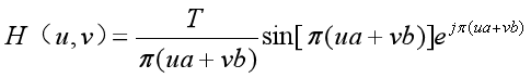 这个退化模型的基本原理大家可以参考一下别的文献,这里就不作介绍了。 这个退化模型的基本原理大家可以参考一下别的文献,这里就不作介绍了。
简单的先退化后复原。
实验原理 设运动图像为f(x,y),其傅里叶变换为F(u,v) 设模糊后的图像为g(x,y),其傅里叶变换为G(u,v) 通过F(u,v)和H(u,v)频域相乘得到G(u,v),即 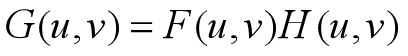 将G(u,v)反变换,就可以得到运动模糊后的图像g(x,y)。 实验结果 将G(u,v)反变换,就可以得到运动模糊后的图像g(x,y)。 实验结果
我们使用H(u,v)模糊图像,其中a = 0,b = 0.1,T = 0.1,得到模糊图像。由多次实验可以得出,参数a是代表竖直方向的位移,参数b代表水平方向的位移。T代表得到图片的曝光时间。  接下来,使用维纳滤波将运动模糊后的图片进行复原。 维纳滤波复原公式如下: 接下来,使用维纳滤波将运动模糊后的图片进行复原。 维纳滤波复原公式如下: 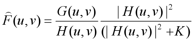 复原结果如下,其中参数和模糊的时候设置的一样,K=1e-4,可以看到哪怕是知道它是用什么样的参数退化的,也很难完美的恢复原图像。 复原结果如下,其中参数和模糊的时候设置的一样,K=1e-4,可以看到哪怕是知道它是用什么样的参数退化的,也很难完美的恢复原图像。 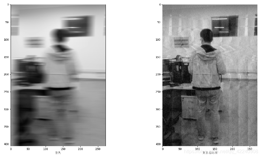
复原拍摄的运动模糊图像
在我们不知道图像时怎么运动模糊的时候,我们需要根据具体图片的退化情况,调节退化模型的参数来得到一个比较好的效果
下面三张图是我们拍摄的需要复原的原图。  维纳滤波法 维纳滤波法
第一张时原图,第二张图时复原的结果,很暗淡,第三张图时经过直方图均衡化后的图,看上去清楚一些。复原结果会由一些竖线条纹,很难去除!
(1)a = 1e-6,b = 0.1,T = 0.1,K = 1e-11时的结果。  (2)a = 1e-6,b = 0.1,T = 0.1,K = 1e-11时的结果 (2)a = 1e-6,b = 0.1,T = 0.1,K = 1e-11时的结果  (3)a = 0.1,b = 1e-6,T = 0.1,K = 1e-11时的结果 (3)a = 0.1,b = 1e-6,T = 0.1,K = 1e-11时的结果  约束最小二乘方滤波法 约束最小二乘方滤波法
约束最小二乘方滤波复原公式: 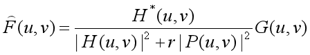 约束最小二乘方滤波的复原结果可以解决竖线条纹的问题,但是结果会相比维纳滤波法稍微模糊一点。 约束最小二乘方滤波的复原结果可以解决竖线条纹的问题,但是结果会相比维纳滤波法稍微模糊一点。
(1)a = 1e-5,b =0.1 ,T = 0.1,r = 0.000005时的结果。  (2)a = 1e-5,b = 0.1,T = 0.1,r = 0.0000005时的结果 (2)a = 1e-5,b = 0.1,T = 0.1,r = 0.0000005时的结果  (3)a = 0.1,b = 1e-4,T = 0.7,r = 0.00001时的结果 (3)a = 0.1,b = 1e-4,T = 0.7,r = 0.00001时的结果  最后把代码分享一下吧。 最后把代码分享一下吧。
# 利用维纳滤波还原图像
import cv2
import numpy as np
from numpy import fft
from matplotlib import pyplot as plt
import cmath
def degradation_function(m, n,a,b,T):
P = m / 2 + 1
Q = n / 2 + 1
Mo = np.zeros((m, n), dtype=complex)
for u in range(m):
for v in range(n):
temp = cmath.pi * ((u - P) * a + (v - Q) * b)
if temp == 0:
Mo[u, v] = T
else:
Mo[u, v] = T * cmath.sin(temp) / temp * cmath.exp(- 1j * temp)
return Mo
def image_mapping(image):
img = image/np.max(image)*255
return img
if __name__ == '__main__':
img = cv2.imread('haogemohu3.png',0)
m, n = img.shape
a = 1e-6
b = 0.1
T = 0.1
K = 1e-11
G = fft.fft2(img)
G_shift = fft.fftshift(G)
H = degradation_function(m, n,a,b,T)
F = G_shift *((np.abs(H)*np.abs(H)) / (H*np.abs(H)*np.abs(H)+K))
f_pic = np.abs(fft.ifft2(F))
res = image_mapping(f_pic)
res1 = res.astype('uint8')
res1 = cv2.medianBlur(res1, 3)
res2 = cv2.equalizeHist(res1)
plt.subplot(131)
plt.imshow(img,cmap='gray')
plt.xlabel('原图', fontproperties='FangSong', fontsize=12)
plt.subplot(132)
plt.imshow(res1,cmap='gray')
plt.xlabel('复原后的图', fontproperties='FangSong', fontsize=12)
plt.subplot(133)
plt.imshow(res2,cmap='gray')
plt.xlabel('复原后的图直方图均衡化', fontproperties='FangSong', fontsize=12)
plt.show()
# 利用最小二乘法复原图像
import cv2
import numpy as np
from numpy import fft
from matplotlib import pyplot as plt
import cmath
def degradation_function(m, n,a,b,T):
P = m / 2 + 1
Q = n / 2 + 1
Mo = np.zeros((m, n), dtype=complex)
for u in range(m):
for v in range(n):
temp = cmath.pi * ((u - P) * a + (v - Q) * b)
if temp == 0:
Mo[u, v] = T
else:
Mo[u, v] = T * cmath.sin(temp) / temp * cmath.exp(- 1j * temp)
return Mo
def image_mapping(image):
img = image/np.max(image)*255
return img
if __name__ == '__main__':
img = cv2.imread('haogemohu3.png',0)
m, n = img.shape
a = 1e-5
b = 0.1
T = 0.1
r = 0.000005
G = fft.fft2(img)
G_shift = fft.fftshift(G)
H = degradation_function(m, n,a,b,T)
p = np.array([[0,-1,0],
[-1,4,-1],
[0,-1,0]])
P = fft.fft2(p,[img.shape[0],img.shape[1]])
F = G_shift *(np.conj(H) / (np.abs(H)**2+r*np.abs(P)**2))
f_pic = np.abs(fft.ifft2(F))
res = image_mapping(f_pic)
res1 = res.astype('uint8')
#res1 = cv2.medianBlur(res1, 3)
res2 = cv2.equalizeHist(res1)
plt.subplot(131)
plt.imshow(img,cmap='gray')
plt.xlabel('原图', fontproperties='FangSong', fontsize=12)
plt.subplot(132)
plt.imshow(res1,cmap='gray')
plt.xlabel('复原后的图', fontproperties='FangSong', fontsize=12)
plt.subplot(133)
plt.imshow(res2,cmap='gray')
plt.xlabel('复原后的图直方图均衡化', fontproperties='FangSong', fontsize=12)
plt.show()
|