数字图像处理 |
您所在的位置:网站首页 › 在matlab中如何对图像对比 › 数字图像处理 |
数字图像处理
|
文章目录
数字图像处理-运动模糊&逆滤波&维纳滤波(Matlab)1、对指定的一幅灰度图像,先用3*3均值滤波器进行模糊处理,形成退化图像1;再叠加椒盐噪声,形成退化图像2;再对上述退化图像1和2采用逆滤波进行复原,给出复原结果图像。分析对比在对H零点问题采用不同处理方法下的复原结果。1-1 图像退化(均值滤波+椒盐噪声)1-2 直接逆滤波还原图像1-3 去掉噪声分量逆滤波还原图像
2、对一幅灰度图像进行运动模糊并叠加高斯噪声,并采用维纳滤波进行复原。2-1 图像退化(运动模糊+高斯噪声)2-2 维纳滤波(Matlab自带函数:deconvwnr)2-3 根据公式编写维纳滤波
数字图像处理-运动模糊&逆滤波&维纳滤波(Matlab)
1、对指定的一幅灰度图像,先用3*3均值滤波器进行模糊处理,形成退化图像1;再叠加椒盐噪声,形成退化图像2;再对上述退化图像1和2采用逆滤波进行复原,给出复原结果图像。分析对比在对H零点问题采用不同处理方法下的复原结果。
1-1 图像退化(均值滤波+椒盐噪声)
Matlab代码块:
%---------------------9x9均值滤波模糊处理-------------------
clc; %清空控制台
clear; %清空工作区
close all; %关闭已打开的figure图像窗口
color_pic=imread('lena512color.bmp'); %读取彩色图像
gray_pic=rgb2gray(color_pic); %将彩色图转换成灰度图
double_gray_pic=im2double(gray_pic); %将uint8转成im2double型便于后期计算
[width,height]=size(double_gray_pic);
H=fspecial('average',9); %生成9x9均值滤波器,图像更模糊,3x3几乎看不出差别
degrade_img1=imfilter(double_gray_pic, H, 'conv', 'circular'); %使用卷积滤波,默认是相关滤波
%--------------------在均值滤波模糊图像基础上添加椒盐噪声------------------
degrade_img2=imnoise(degrade_img1,'salt & pepper',0.05); %给退化图像1添加噪声密度为0.05的椒盐噪声(退化图像2)
figure('name','退化图像');
subplot(2,2,1);imshow(color_pic,[]);title('原彩色图');
subplot(2,2,2);imshow(double_gray_pic,[]);title('原灰度图');
subplot(2,2,3);imshow(degrade_img1,[]);title('退化图像1');
subplot(2,2,4);imshow(degrade_img2,[]);title('退化图像2');
运行效果:
 1-3 去掉噪声分量逆滤波还原图像
Matlab代码块:
%------------------------去掉噪声分量逆滤波复原-----------------------
noise=degrade_img2-degrade_img1; %提取噪声分量
fourier_noise=fft2(noise); %对噪声进行傅里叶变换
restore_three=ifft2((fourier_degrade_img2-fourier_noise)./fourier_H); %G(u,v)=H(u,v)F(u,v)+N(u,v),解得F(u,v)=[G(u,v)-N(u,v)]/H(u,v)
figure('name','退化图像2逆滤波复原');
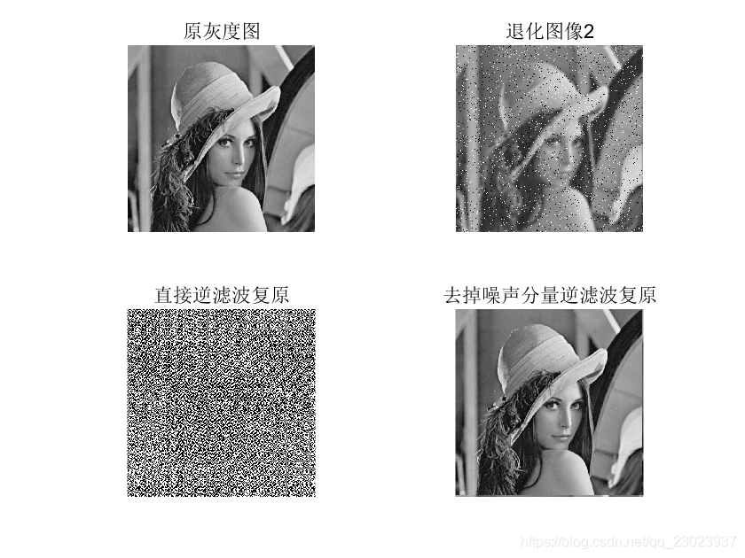
subplot(2,2,1);imshow(double_gray_pic,[]);title('原灰度图');
subplot(2,2,2);imshow(im2uint8(degrade_img2),[]);title('退化图像2');
subplot(2,2,3);imshow(im2uint8(restore_two),[]);title('直接逆滤波复原');
subplot(2,2,4);imshow(im2uint8(restore_three),[]);title('去掉噪声分量逆滤波复原');
运行效果:
1-3 去掉噪声分量逆滤波还原图像
Matlab代码块:
%------------------------去掉噪声分量逆滤波复原-----------------------
noise=degrade_img2-degrade_img1; %提取噪声分量
fourier_noise=fft2(noise); %对噪声进行傅里叶变换
restore_three=ifft2((fourier_degrade_img2-fourier_noise)./fourier_H); %G(u,v)=H(u,v)F(u,v)+N(u,v),解得F(u,v)=[G(u,v)-N(u,v)]/H(u,v)
figure('name','退化图像2逆滤波复原');
subplot(2,2,1);imshow(double_gray_pic,[]);title('原灰度图');
subplot(2,2,2);imshow(im2uint8(degrade_img2),[]);title('退化图像2');
subplot(2,2,3);imshow(im2uint8(restore_two),[]);title('直接逆滤波复原');
subplot(2,2,4);imshow(im2uint8(restore_three),[]);title('去掉噪声分量逆滤波复原');
运行效果:
G ( u , v ) = H ( u , v ) F ( u , v ) + N ( u , v ) G(u,v)=H(u,v)F(u,v)+N(u,v) G(u,v)=H(u,v)F(u,v)+N(u,v) G ( u , v ) H ( u , v ) = F ( u , v ) + N ( u , v ) H ( u , v ) \dfrac{G(u,v)}{H(u,v)}=F(u,v)+\dfrac{N(u,v)}{H(u,v)} H(u,v)G(u,v)=F(u,v)+H(u,v)N(u,v) 从上式可见,如果H(u,v)足够小,则输出结果被噪声所支配,复原出来的图像便是一幅充满椒盐噪声的图。 所以当我们已知道所加的噪声信号时,还原出的信号为 F ( u , v ) = G ( u , v ) − N ( u , v ) H ( u , v ) F(u,v)=\dfrac{G(u,v)-N(u,v)}{H(u,v)} F(u,v)=H(u,v)G(u,v)−N(u,v),即如果不知道噪声信号,则清晰还原困难。 2、对一幅灰度图像进行运动模糊并叠加高斯噪声,并采用维纳滤波进行复原。 2-1 图像退化(运动模糊+高斯噪声) Matlab代码块: % ----------------2、对一幅灰度图像进行运动模糊并叠加高斯噪声,并采用维纳滤波进行复原------------- clc; %清空控制台 clear; %清空工作区 close all; %关闭已打开的figure图像窗口 color_pic=imread('lena512color.bmp'); %读取彩色图像 gray_pic=rgb2gray(color_pic); %将彩色图转换成灰度图 double_gray_pic=im2double(gray_pic); %将uint8转成im2double型便于后期计算 [width,height]=size(double_gray_pic); %-------------------------添加运动模糊---------------------- H_motion = fspecial('motion', 18, 90);%运动长度为18,逆时针运动角度为90° motion_blur = imfilter(double_gray_pic, H_motion, 'conv', 'circular');%卷积滤波 noise_mean=0; %添加均值为0 noise_var=0.001; %方差为0.001的高斯噪声 motion_blur_noise=imnoise(motion_blur,'gaussian',noise_mean,noise_var);%添加均值为0,方差为0.001的高斯噪声 figure('name','运动模糊加噪'); subplot(1,2,1);imshow(motion_blur,[]);title('运动模糊'); subplot(1,2,2);imshow(motion_blur_noise,[]);title('运动模糊添加噪声'); 运行效果:
J = deconvwnr(I,PSF,NSR) deconvolves image I using the Wiener filter algorithm, returning deblurred image J. Image I can be an N-dimensional array. PSF is the point-spread function with which I was convolved. NSR is the noise-to-signal power ratio of the additive noise. NSR can be a scalar or a spectral-domain array of the same size as I. Specifying 0 for the NSR is equivalent to creating an ideal inverse filter. Matlab代码块: %----------------------------维纳滤波matlab自带函数deconvwnr------------------------- restore_ignore_noise = deconvwnr(motion_blur_noise, H_motion, 0); %nsr=0,忽视噪声 signal_var=var(double_gray_pic(:)); estimate_nsr=noise_var/signal_var; %噪信比估值 restore_with_noise=deconvwnr(motion_blur_noise,H_motion,estimate_nsr); %信号的功率谱使用图像的方差近似估计 figure('name','函数法维纳滤波'); subplot(1,2,1);imshow(im2uint8(restore_ignore_noise),[]);title('忽视噪声直接维纳滤波(nsr=0),相当于逆滤波'); subplot(1,2,2);imshow(im2uint8(restore_with_noise),[]);title('考虑噪声维纳滤波'); 运行效果:
|


【本文地址】
今日新闻 |
推荐新闻 |