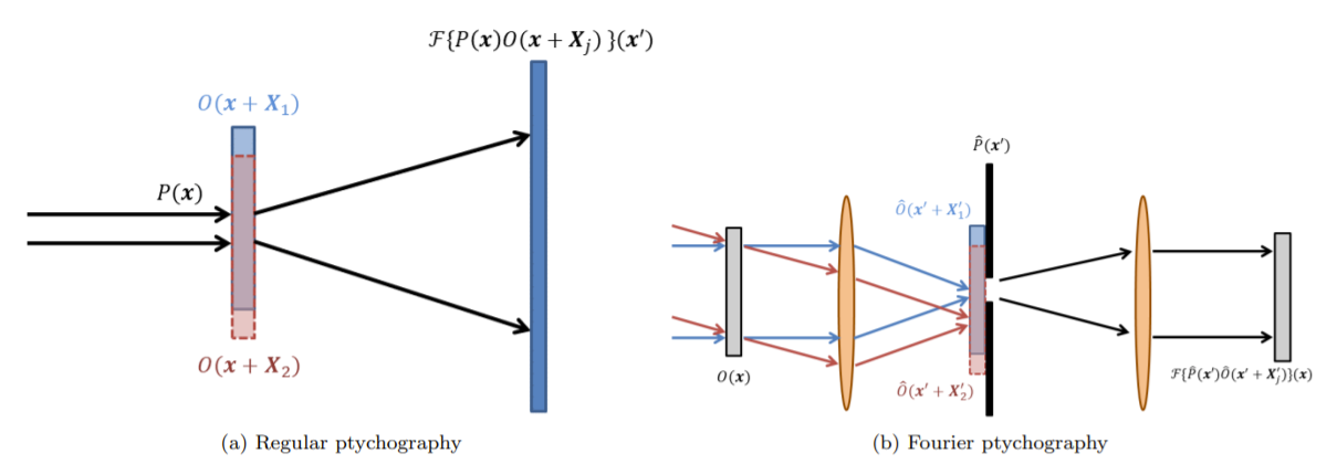
参考论文： Konijnenberg, S. (2017). An introduction to the theory of ptychographic phase retrieval methods. Advanced Optical Technologies, 6(6), 423–438. https://doi.org/10.1515/aot-2017-0049

物理学问题：我们对波的测量是有限制的，具体来说，比如有一个单色光\(U=|U| e^{i \phi}\)，我们其实只能测量\(U^2\)，不能测量\(\phi\)（phase）。

干涉法间接得到相位：two fields \(U_{1}=\left|U_{1}\right| e^{i \phi_{1}}\) and \(U_{2}=\left|U_{2}\right| e^{i \phi_{2}}\)，观察到的强度是：

这个技术的问题：笨重，容易被扰动（甚至因此可以用来测量地球引力）

有：a complex-valued transmission function \(\psi(\mathbf{x})\)，its Fourier transform as \(\Psi\left(\mathbf{x}^{\prime}\right)\)，the intensity pattern measured in the far field \(\left|\Psi\left(\mathbf{x}^{\prime}\right)\right|^{2}\) 那么有两个对 \(\psi(\mathbf{x})\)的约束：

那么可以用ER（error reduction）算法，在两个domain之间反复横跳进行调整，迭代地更新 \(\psi(\mathbf{x})\)。文章接着对ER算法从 feasibility problem 和 cost minimization problem 的角度进行了证明和解释，并且从这两个角度可以分别进行算法的改良。

用多个wave。 其中一个wave：

照亮未知的物体O(x) with a known probe P(x) that is shifted to different positions Xj 同样可以用ER算法去迭代更新，因为重叠部分的存在能够更鲁棒。

计算O(x)的傅里叶变换\(\hat{O}\left(\mathbf{x}^{\prime}\right)\)而不是它本身。

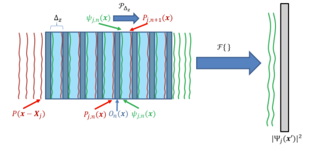
前面的公式基于物体是薄片的假设。 multislice method：把3D物体假设成很多切片，每一片满足薄物体假设

在第n个slice，入射波为：

可以递归地定义出射光：

3D Fourier ptychography：

\(v(\mathbf{x})\)是要重建的3D信息，\(V\left(\mathbf{x}^{\prime}\right)\)是它的傅里叶变换，\(\mathbf{k}_{\text {scat }}\) 是长度为\(\frac{1}{\lambda}\)指向散射方向的向量，\(\mathbf{k}_{\text {inc }}\)指向入射光方向，则：

改变入射光方向 \(\mathbf{k}_{\text {inc }}\)就可以探测物体的不同部分。

个人理解和补充：通篇最没有理解清楚的一点是：为什么采集到的是傅里叶变换的结果。没有查到衍射成像的原理，参考知乎：简单认识傅里叶光学，最重要的一句话：当以单色平面波垂直照明透镜前焦面的样品时，在透镜后焦面上的分布，正比于样品复振幅分布的傅里叶变换。以及这篇专栏，最重要的一句话：对于Fraunhoffer衍射光的强度是孔径函数傅里叶变换的幅值。通过这两句话能够勉强理解论文的逻辑。不过物理学比较无所谓...总之就是有了新的deconvolution的思路，是ER方法以及后面的数学分析，以及有了一点点从衍射出发的思路。