|
一、气泡图
第一种会放success和speed的图,然后圆圈的大小是结合两者综合后的性能,俗称“气泡图” 先放一下自己模仿ocean画的一幅图:
 以下是画的代码(直接运行就能出来上面这幅图): 以下是画的代码(直接运行就能出来上面这幅图):
import numpy as np
import matplotlib.pyplot as plt
import matplotlib.axes._axes as axes
import matplotlib.figure as figure
from matplotlib.backends.backend_pdf import PdfPages
pdf = PdfPages('speed-eao2018.pdf')
plt.rc('font',family='Times New Roman')
fig, ax = plt.subplots() # type:figure.Figure, axes.Axes
ax.set_title('The Performance $vs.$ Speed on VOT-2018', fontsize=15)
ax.set_xlabel('Tracking Speed (FPS)', fontsize=15)
ax.set_ylabel('EAO', fontsize=15)
trackers = ['C-RPN', 'SiamVGG', 'DaSiamRPN', 'ATOM', 'SiamRPN++', 'DiMP', 'Ours (offline-2)', 'Ours (offline-1)', 'Ours (online)']
speed = np.array([50, 75, 65, 35, 50, 45, 72, 58, 25])
speed_norm = np.array([50, 75, 65, 35, 50, 45, 72, 58, 25]) / 48
performance = np.array([0.273, 0.286, 0.380, 0.401, 0.414, 0.440, 0.438, 0.467, 0.490])
circle_color = ['cornflowerblue', 'deepskyblue', 'turquoise', 'gold', 'yellowgreen', 'orange', 'r', 'r', 'r']
# Marker size in units of points^2
volume = (300 * speed_norm/5 * performance/0.6) ** 2
ax.scatter(speed, performance, c=circle_color, s=volume, alpha=0.4)
ax.scatter(speed, performance, c=circle_color, s=20, marker='o')
# text
ax.text(speed[0] - 2.37, performance[0] - 0.031, trackers[0], fontsize=10, color='k')
ax.text(speed[1] - 11.00, performance[1] - 0.005, trackers[1], fontsize=10, color='k')
ax.text(speed[2] - 3.5, performance[2] - 0.05, trackers[2], fontsize=10, color='k')
ax.text(speed[3] - 2.4, performance[3] - 0.032, trackers[3], fontsize=10, color='k')
ax.text(speed[4] - 2.9, performance[4] - 0.040, trackers[4], fontsize=10, color='k')
ax.text(speed[5] - 1.8, performance[5] - 0.042, trackers[5], fontsize=10, color='k')
ax.text(speed[6] - 6.0, performance[6] + 0.051, trackers[6], fontsize=14, color='k')
ax.text(speed[7] - 4.5, performance[7] -0.050, trackers[7], fontsize=12, color='k')
ax.text(speed[8] - 4, performance[8] -0.035, trackers[8], fontsize=12, color='k')
ax.grid(which='major', axis='both', linestyle='-.') # color='r', linestyle='-', linewidth=2
ax.set_xlim(20, 80)
ax.set_ylim(0.20, 0.53)
ax.xaxis.set_tick_params(labelsize=15)
ax.yaxis.set_tick_params(labelsize=15)
# plot lines
ystart, yend = ax.get_ylim()
ax.plot([25, 25], [ystart, yend], linestyle="--", color='k', linewidth=0.7)
ax.plot([25, 58], [0.490, 0.467], linestyle="--", color='r', linewidth=0.7)
ax.plot([58, 72], [0.467, 0.438], linestyle="--", color='r', linewidth=0.7)
ax.text(26, 0.230, 'Real-time line', fontsize=11, color='k')
fig.savefig('speed-eao2018.svg')
pdf.savefig()
pdf.close()
plt.show()
主要要提供的就是每个tracker的speed和success,其他字的位置和圈的相对大小都是自己调整的
二、vot_eao_rank图
这主要是画vot的eao排序的图,代码来自于这里
 matlab代码长这样: matlab代码长这样:
clear; close all; clc;
load('../data/attr_eao_vot2016.mat');
tracker_names = fieldnames(result);
legend_names = fieldnames(result.(tracker_names{1}));
num_tracker = length(tracker_names);
num_attr = length(legend_names);
eao = zeros(num_tracker,num_attr);
for i = 1:num_tracker
for j = 1:num_attr
eao(i,j) = result.(tracker_names{i}).(legend_names{j});
end
end
[eao_sorted,sorted_index] = sort(eao(:,1),'descend'); % rank by baseline eao
tracker_names = tracker_names(sorted_index);
figure;
Maker_style = {'o','x','*','v','diamond','+','','square','^','hexagram'};
Color_style = hsv(7);
line([0,num_tracker],[0.255,0.255],'LineWidth',2,'Color',[0.7 0.7 0.7]); hold on;
recent_index = [1,2,4,5,7,10,13,15,17,22,28,31,36,39,50];
for i = 1:num_tracker
if i == 1 || i == 3
m(i) = plot(i,eao_sorted(i),'Marker','.','Color',Color_style(i,:),...
'LineStyle','none','LineWidth',2,'MarkerSize',35);hold on;
else
m(i) = plot(i,eao_sorted(i),'Marker',Maker_style{mod(i-1,12)+1},'Color',Color_style(mod(i-1,7)+1,:),...
'LineStyle','none','LineWidth',2,'MarkerSize',10);hold on;
end
plot([i,i],[0,eao_sorted(i)],'LineStyle',':','Color',[0.83 0.81 0.78]);hold on;
if any(i == recent_index)
plot(i+2, 0.05,'MarkerSize',6,'Marker','o','LineStyle','none',...
'Color',[0.83 0.81 0.8],'LineWidth',2);hold on;
end
end
set(gca,'xdir','reverse')
ylim([0,(eao_sorted(1)+0.05)]);
xlim([1, num_tracker]);
set(gca,'XTick',1:5:70);
set(gca,'YTick',0:0.05:(eao_sorted(1)+0.05))
set(gca,'linewidth',2);
set(gca,'FontSize',12);
% annotation('textarrow',[0.76,0.8],[0.76,0.72],'String','SAECO','FontWeight','bold','FontSize',12);
annotation('textbox',[.15,.8,.1,.1],'String','$$\hat{\Phi}$$','FontWeight','bold','FontSize',30,'LineStyle','none','Interpreter','latex','FitBoxToText','off')
box on
num_tracker_show = 10; % only write top10
for i = 1:num_tracker_show %
legend_names{i} = [strrep(tracker_names{i},'_','\_'),...
num2str(eao_sorted(i),'~[%0.3f]')];
end
legend(m(1:num_tracker_show),legend_names(1:num_tracker_show),...
'Location','eastoutside','Interpreter', 'latex','FontSize',16)
set(gcf, 'position', [500 300 800 250]);
saveas(gcf,'../img/eao_rank_vot2016','pdf');
saveas(gcf,'../img/eao_rank_vot2016','png');
最主要的也是先要有这个attr_eao_vot2016.mat,也就是每个tracker在vot的每个属性以及overall的结果。
三、属性雷达图
这还得来自于有属性挑战的数据集上的结果,比如LaSOT,VOT,OTB等,现在的代码是来自于这里,在matlab底下画出来的,先看一下效果图:  然后上代码: 然后上代码:
clear; close all; clc;
load('../data/attr_eao_vot2016.mat');
tracker_names = fieldnames(result);
legend_names = fieldnames(result.(tracker_names{1}));
num_tracker = length(tracker_names);
num_attr = length(legend_names);
eao = zeros(num_tracker,num_attr);
for i = 1:num_tracker
for j = 1:num_attr
eao(i,j) = result.(tracker_names{i}).(legend_names{j});
end
end
[s,sorted_index] = sort(eao(:,1),'descend'); % rank by baseline eao
num_tracker_show = 10; % only write top10
tracker_names = tracker_names(sorted_index(1:num_tracker_show));
eao = eao(sorted_index(1:num_tracker_show),:);
eao(:,num_attr+1) = eao(:,1);
a_min = min(eao,[],1);
a_max = max(eao,[],1);
t = (0:1/num_attr:1)*2*pi;
h = [];
masker_shape = {'x','.'};
masker_size = {10,40};
color_masker = hsv(num_tracker_show);
color_line = color_masker*0.4 +ones(num_tracker_show,3)*0.6;
ax = polaraxes;
for i = 1:num_tracker_show
h(i) = polarplot(t, (eao(i,:)-a_min)./(a_max-a_min)+0.2, 'MarkerSize',masker_size{mod(i,2)+1},...
'Marker',masker_shape{mod(i,2)+1},'LineWidth',2,...
'Color',color_line(i,:),'MarkerEdgeColor',color_masker(i,:)); hold on;
end
polarplot(t, 0.5, 'LineWidth',2, 'Color',[0,0,0]); hold on;
grid off
legend_names = {'Overall','Occlusion','Camera~motion','Size~change',...
'Illumination~change','Motion~change', 'Unassigned'};
for i = 1:num_attr
legend_names{i} = ['\begin{tabular}{c}', legend_names{i}, '\\',...
[num2str(a_min(i),'(%.3f,') num2str(a_max(i),'%.3f)')], '\end{tabular}'];
end
ax.ThetaTickLabels = legend_names;
ThetaTick = (0:1/num_attr:1)*360;
ax.ThetaTick = ThetaTick(1:end-1);
ax.RTickLabels = [];
ax.TickLabelInterpreter = 'latex';
for i = 1:num_tracker_show %
tracker_names{i} = strrep(tracker_names{i},'_','\_');
end
ah1 = gca;
legend1=legend(ah1,h(1:5),tracker_names(1:5),'Orientation','horizontal','Location','southoutside');
ah2=axes('position',get(gca,'position'), 'visible','off');
legend2=legend(ah2,h(6:10),tracker_names(6:10),'Orientation','horizontal','Location','southoutside');
set(legend1,'Box','off')
set(legend2,'Box','off')
legend1_pos = get(legend1,'Position');
set(legend2,'Position',legend1_pos-[0,legend1_pos(4)*1.2,0,0]);
% set(gcf, 'position', [500 300 800 800]);
saveas(gcf,'../img/attr_eao_vot2016','pdf')
saveas(gcf,'../img/attr_eao_vot2016','png')
四、属性雷达图画法2
下面画的是在LasHeR上各个属性挑战下的成功率雷达图,出处在这里,可以直接在python底下运行,先看一下效果图: 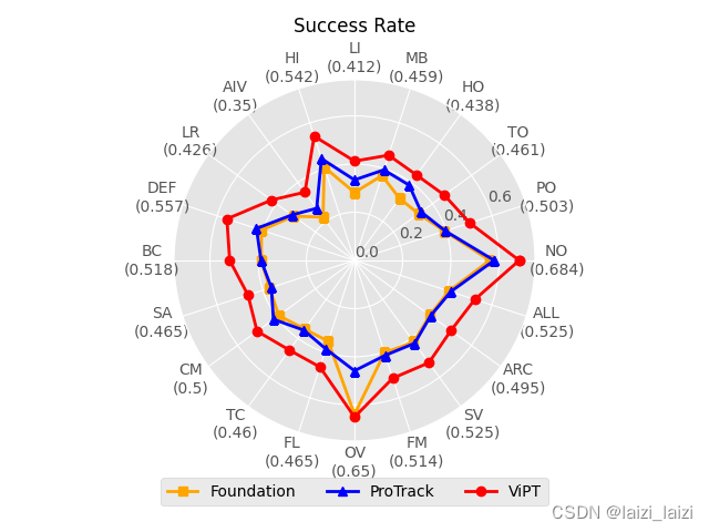 直接上代码,大家有需要就是属性结果和算法名称部分自己修改一下即可: 直接上代码,大家有需要就是属性结果和算法名称部分自己修改一下即可:
import numpy as np
import matplotlib.pyplot as plt
plt.style.use('ggplot')
foundation = [0.562, 0.393, 0.329, 0.318, 0.370, 0.282, 0.407, 0.222, 0.312, 0.406, 0.387, 0.370, 0.389, 0.352, 0.353, 0.639, 0.403, 0.418, 0.387, 0.412]
protrack = [0.580, 0.396, 0.342, 0.386, 0.395, 0.334, 0.444, 0.267, 0.321, 0.428, 0.388, 0.363, 0.416, 0.358, 0.386, 0.458, 0.414, 0.425, 0.391, 0.420]
ViPT = [0.684, 0.503, 0.461, 0.438, 0.459, 0.412, 0.542, 0.350, 0.426, 0.557, 0.518, 0.465, 0.500, 0.460, 0.465, 0.650, 0.514, 0.525, 0.495, 0.525]
feature = ['NO', 'PO', 'TO', 'HO', 'MB', 'LI', 'HI', 'AIV', 'LR', 'DEF', 'BC', 'SA', 'CM', 'TC', 'FL', 'OV', 'FM', 'SV', 'ARC', 'ALL']
angles = np.linspace(0, 2 * np.pi, len(feature), endpoint=False)
fig = plt.figure()
ax = fig.add_subplot(111, polar=True)
ax.plot(np.concatenate((angles, [angles[0]])), np.concatenate((foundation, [foundation[0]])), 's-', linewidth=2, label='Foundation',color='orange')
ax.plot(np.concatenate((angles, [angles[0]])), np.concatenate((protrack, [protrack[0]])), '^-', linewidth=2, label='ProTrack',color='blue')
ax.plot(np.concatenate((angles, [angles[0]])), np.concatenate((ViPT, [ViPT[0]])), 'o-', linewidth=2, label='ViPT',color='red')
logo=[str(x)+'\n'+'('+str(ViPT[i])+')' for i,x in enumerate(feature)]
ax.set_thetagrids(angles * 180 / np.pi, logo)
ax.set_ylim(0, 0.75)
ax.set_yticks([0,0.2,0.4,0.6])
plt.title('Success Rate', fontsize=12)
plt.legend(loc='lower center', prop={'size':10},ncol=4, bbox_to_anchor=[0.5,-0.2]) # 控制图标的居中和往下的距离
ax.grid(True)
plt.show()
最主要的也是先要有这个attr_eao_vot2016.mat,也就是每个tracker在vot的每个属性以及overall的结果。 PS: (1) 有很多人在问怎么得到在VOT上的各属性的EAO值,这里解答一下: 可以使用pysot里面的toolkit,只需要修改这里的tags=[‘all,camera_motion,illum_change,motion_change,size_change,occlusion,empty’],其中empty得分就是上面雷达图中的Unassigned 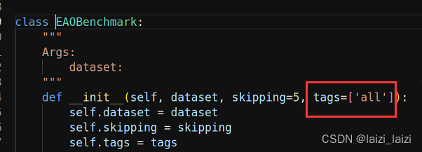 (2) 那得到了VOT上的各属性的EAO值,怎么生成attr_eao_vot2016.mat文件,这里也提供一下生成的matlab代码: 脚本名为generate_attr_eao.m,这里仅以SiamFC和MDNet算法举例,自己想要添加啥都以此类推。 (2) 那得到了VOT上的各属性的EAO值,怎么生成attr_eao_vot2016.mat文件,这里也提供一下生成的matlab代码: 脚本名为generate_attr_eao.m,这里仅以SiamFC和MDNet算法举例,自己想要添加啥都以此类推。
%%%%% SiamFC %%%
SiamFC.all = 0.234;
SiamFC.occlusion = 0.161;
SiamFC.motion_change = 0.191;
SiamFC.size_change = 0.242;
SiamFC.illum_change = 0.180;
SiamFC.camera_motion = 0.231;
SiamFC.empty = 0.059;
%%%%% MDNet %%%
MDNet.all = 0.257;
MDNet.occlusion = 0.218;
MDNet.motion_change = 0.238;
MDNet.size_change = 0.312;
MDNet.illum_change = 0.313;
MDNet.camera_motion = 0.252;
MDNet.empty = 0.030;
result.SiamFC = SiamFC;
result.MDNet = MDNet;
save(['attr_eao_vot2016.mat'], 'result');
|