Python 数据分析实战案例：用户行为预测

您所在的位置：网站首页 › 各种sans介绍图 › Python 数据分析实战案例：用户行为预测

Python 数据分析实战案例：用户行为预测

2023-03-03 22:17| 来源: 网络整理| 查看: 265

文章目录案例介绍技术提升读取数据数据预处理数据探索与可视化数据分析用户流量和购买时间情况分析总访问量成交量时间变化分析(天)总访问量成交量时间变化分析(小时) 特征工程行为类型点击次数加购次数收藏次数相关分析数据标签建立模型逻辑回归模型评估随机森林模型评估

案例介绍

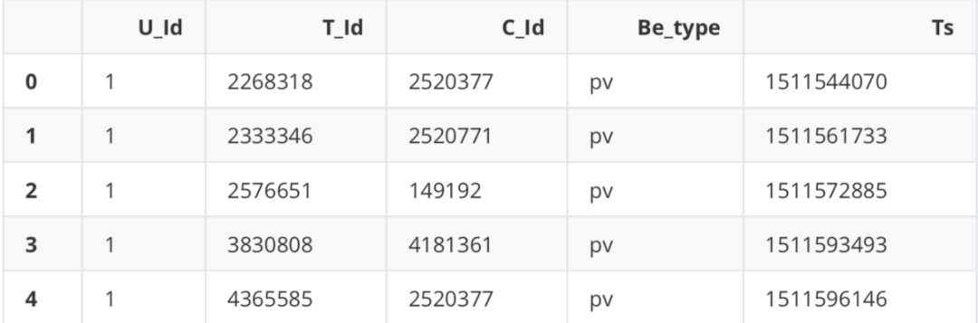
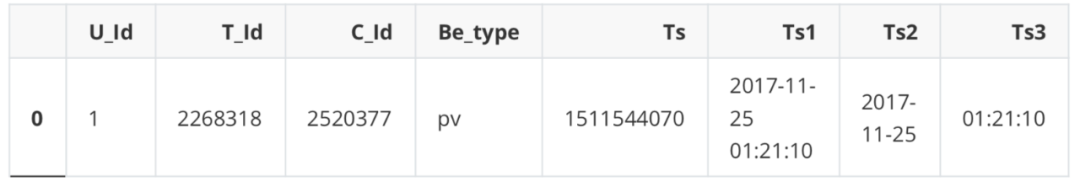
背景：以某大型电商平台的用户行为数据为数据集，使用大数据处理技术分析海量数据下的用户行为特征，并通过建立逻辑回归模型、随机森林对用户行为做出预测;

案例思路:

使用大数据处理技术读取海量数据

海量数据预处理

抽取部分数据调试模型

使用海量数据搭建模型

技术提升

技术要学会分享、交流，不建议闭门造车。一个人可以走的很快、一堆人可以走的更远。

文中源码、资料分享、数据、技术交流提升，均可加交流群获取，群友已超过2000人，添加时最好的备注方式为：来源+兴趣方向，方便找到志同道合的朋友。

方式①、添加微信号：pythoner666，备注：来自CSDN 方式②、微信搜索公众号：Python学习与数据挖掘，后台回复：加群

#全部行输出 from IPython.core.interactiveshell import InteractiveShell InteractiveShell.ast_node_interactivity = "all"

数据字典:

U_Id:the serialized ID that represents a user

T_Id:the serialized ID that represents an item

C_Id:the serialized ID that represents the category which the corresponding item belongs to Ts:the timestamp of the behavior

Be_type:enum-type from (‘pv’, ‘buy’, ‘cart’, ‘fav’)

pv: Page view of an item’s detail page, equivalent to an item click

_buy: Purchase an item _

cart: Add an item to shopping cart fav: Favor an item

读取数据

这里关键是使用dask库来处理海量数据，它的大多数操作的运行速度比常规pandas等库快十倍左右。

pandas在分析结构化数据方面非常的流行和强大，但是它最大的限制就在于设计时没有考虑到可伸缩性。pandas特别适合处理小型结构化数据，并且经过高度优化，可以对存储在内存中的数据执行快速高效的操作。然而随着数据量的大幅度增加，单机肯定会读取不下的，通过集群的方式来处理是最好的选择。这就是Dask DataFrame API发挥作用的地方:通过为pandas提供一个包装器，可以智能的将巨大的DataFrame分隔成更小的片段，并将它们分散到多个worker(帧)中，并存储在磁盘中而不是RAM中。

Dask DataFrame会被分割成多个部门，每个部分称之为一个分区，每个分区都是一个相对较小的 DataFrame，可以分配给任意的worker，并在需要复制时维护其完整数据。具体操作就是对每个分区并行或单独操作(多个机器的话也可以并行)，然后再将结果合并，其实从直观上也能推出Dask肯定是这么做的。

# 安装库(清华镜像) # pip install dask -i https://pypi.tuna.tsinghua.edu.cn/simple import os import gc # 垃圾回收接口 from tqdm import tqdm # 进度条库 import dask # 并行计算接口 from dask.diagnostics import ProgressBar import numpy as np import pandas as pd import matplotlib.pyplot as plt import time import dask.dataframe as dd # dask中的数表处理库 import sys # 外部参数获取接口

面对海量数据，跑完一个模块的代码就可以加一行gc.collect()来做内存碎片回收，Dask Dataframes与Pandas Dataframes具有相同的API

gc.collect() 42 # 加载数据 data = dd.read_csv('UserBehavior_all.csv')# 需要时可以设置blocksize=参数来手工指定划分方法，默认是64MB(需要设置为总线的倍数，否则会放慢速度) data.head()

data

Dask DataFrame Structure :

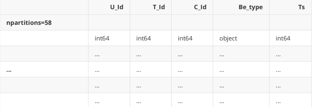
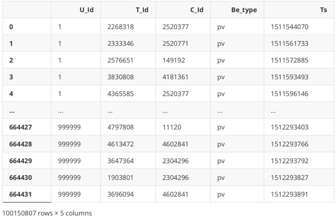
Dask Name: read-csv, 58 tasks

与pandas不同，这里我们仅获取数据框的结构，而不是实际数据框。Dask已将数据帧分为几块加载，这些块存在于磁盘上，而不存在于RAM中。如果必须输出数据帧，则首先需要将所有数据帧都放入RAM，将它们缝合在一起，然后展示最终的数据帧。使用.compute()强迫它这样做，否则它不.compute() 。其实dask使用了一种延迟数据加载机制，这种延迟机制类似于python的迭代器组件，只有当需要使用数据的时候才会去真正加载数据。

# 真正加载数据 data.compute()

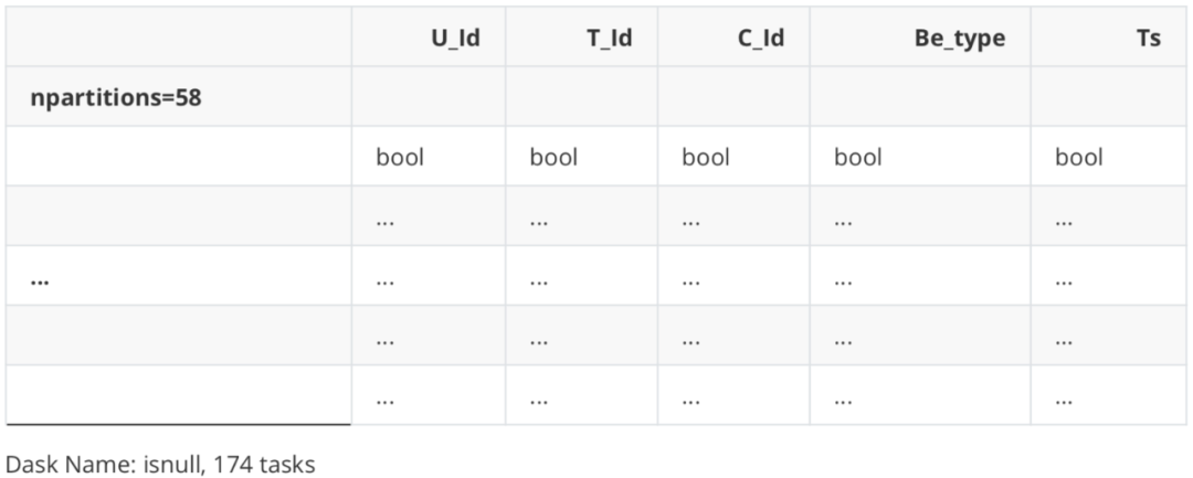
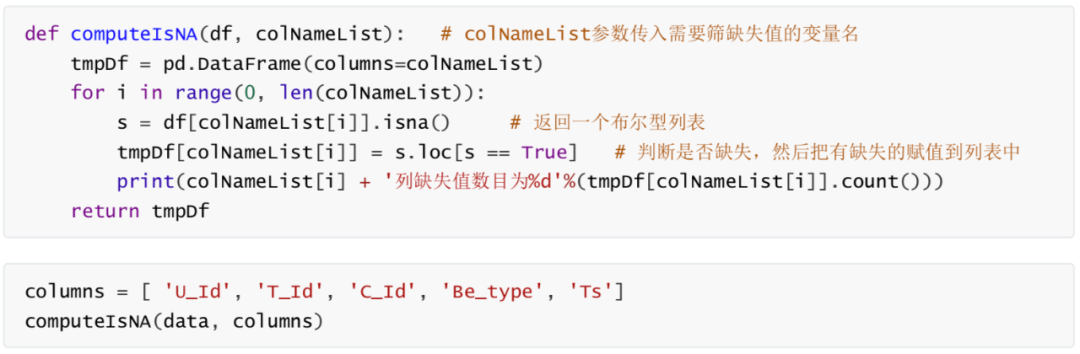
# 可视化工作进程，58个分区任务 data.visualize() 数据预处理

数据压缩

# 查看现在的数据类型 data.dtypes U_Id int64 T_Id int64 C_Id int64 Be_type object Ts int64 dtype: object # 压缩成32位uint，无符号整型，因为交易数据没有负数 dtypes = { 'U_Id': 'uint32', 'T_Id': 'uint32', 'C_Id': 'uint32', 'Be_type': 'object', 'Ts': 'int64' } data = data.astype(dtypes) data.dtypes U_Id uint32 T_Id uint32 C_Id uint32 Be_type object Ts int64 dtype: object

缺失值

# 以dask接口读取的数据，无法直接用.isnull()等pandas常用函数筛查缺失值` ` data.isnull()

Dask DataFrame Structure :

columns1 = [ 'U_Id', 'T_Id', 'C_Id', 'Be_type', 'Ts'] tmpDf1 = pd.DataFrame(columns=columns1) tmpDf1 .dataframe tbody tr th { vertical-align: top; } .dataframe thead th { text-align: right; }

s = data["U_Id"].isna() s.loc[s == True] Dask Series Structure: npartitions=58 bool ... ... ... ... Name: U_Id, dtype: bool Dask Name: loc-series, 348 tasks

U_Id列缺失值数目为0 T_Id列缺失值数目为0 C_Id列缺失值数目为0 Be_type列缺失值数目为0 Ts列缺失值数目为0 数据探索与可视化

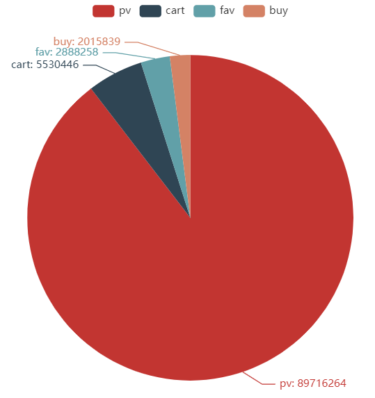
这里我们使用pyecharts库。pyecharts是一款将python与百度开源的echarts结合的数据可视化工具。新版的1.X和旧版的0.5.X版本代码规则大不相同，新版详见官方文档_https://gallery.pyecharts.org/#/README_

# pip install pyecharts -i https://pypi.tuna.tsinghua.edu.cn/simple Looking in indexes: https://pypi.tuna.tsinghua.edu.cn/simple Requirement already satisfied: pyecharts in d:\anaconda\lib\site-packages (0.1.9.4) Requirement already satisfied: jinja2 in d:\anaconda\lib\site-packages (from pyecharts) (3.0.2) Requirement already satisfied: future in d:\anaconda\lib\site-packages (from pyecharts) (0.18.2) Requirement already satisfied: pillow in d:\anaconda\lib\site-packages (from pyecharts) (8.3.2) Requirement already satisfied: MarkupSafe>=2.0 in d:\anaconda\lib\site-packages (from jinja2->pyecharts) (2.0.1) Note: you may need to restart the kernel to use updated packages. U_Id列缺失值数目为0 T_Id列缺失值数目为0 C_Id列缺失值数目为0 Be_type列缺失值数目为0 Ts列缺失值数目为0 WARNING: Ignoring invalid distribution -umpy (d:\anaconda\lib\site-packages) WARNING: Ignoring invalid distribution -ip (d:\anaconda\lib\site-packages) WARNING: Ignoring invalid distribution -umpy (d:\anaconda\lib\site-packages) WARNING: Ignoring invalid distribution -ip (d:\anaconda\lib\site-packages) WARNING: Ignoring invalid distribution -umpy (d:\anaconda\lib\site-packages) WARNING: Ignoring invalid distribution -ip (d:\anaconda\lib\site-packages) WARNING: Ignoring invalid distribution -umpy (d:\anaconda\lib\site-packages) WARNING: Ignoring invalid distribution -ip (d:\anaconda\lib\site-packages) WARNING: Ignoring invalid distribution -umpy (d:\anaconda\lib\site-packages) WARNING: Ignoring invalid distribution -ip (d:\anaconda\lib\site-packages)

饼图

# 例如，我们想画一张漂亮的饼图来看各种用户行为的占比 data["Be_type"]

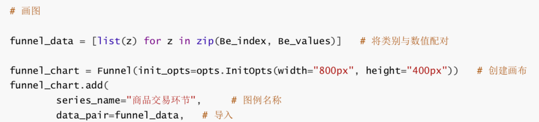
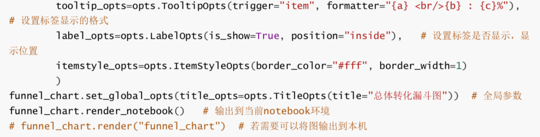
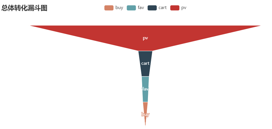
# 使用dask的时候，所有支持的原pandas的函数后面需加.compute()才能最终执行 Be_counts = data["Be_type"].value_counts().compute() Be_counts pv 89716264 cart 5530446 fav 2888258 buy 2015839 Name: Be_type, dtype: int64 Be_index = Be_counts.index.tolist() # 提取标签 Be_index ['pv', 'cart', 'fav', 'buy'] Be_values = Be_counts.values.tolist() # 提取数值 Be_values [89716264, 5530446, 2888258, 2015839] from pyecharts import options as opts from pyecharts.charts import Pie #pie这个包里的数据必须传入由元组组成的列表 c = Pie() c.add("", [list(z) for z in zip(Be_index, Be_values)]) # zip函数的作用是将可迭代对象打包成一个个元组，然后返回这些元组组成的列表 c.set_global_opts(title_opts=opts.TitleOpts(title="用户行为")) # 全局参数(图命名) c.set_series_opts(label_opts=opts.LabelOpts(formatter="{b}: {c}")) c.render_notebook() # 输出到当前notebook环境 # c.render("pie_base.html") # 若需要可以将图输出到本机

漏斗图

from pyecharts.charts import Funnel # 旧版的pyecharts不需要.charts即可import import pyecharts.options as opts from IPython.display import Image as IMG from pyecharts import options as opts from pyecharts.charts import Pie

数据分析

时间戳转换

dask对于时间戳的支持非常不友好

type(data) dask.dataframe.core.DataFrame data['Ts1']=data['Ts'].apply(lambda x: time.strftime("%Y-%m-%d %H:%M:%S", time.localtime(x))) data['Ts2']=data['Ts'].apply(lambda x: time.strftime("%Y-%m-%d", time.localtime(x))) data['Ts3']=data['Ts'].apply(lambda x: time.strftime("%H:%M:%S", time.localtime(x))) D:\anaconda\lib\site-packages\dask\dataframe\core.py:3701: UserWarning: You did not provide metadata, so Dask is running your function on a small dataset to guess output types. It is possible that Dask will guess incorrectly. To provide an explicit output types or to silence this message, please provide the `meta=` keyword, as described in the map or apply function that you are using. Before: .apply(func) After: .apply(func, meta=('Ts', 'object')) warnings.warn(meta_warning(meta)) data.head(1)

data.dtypes U_Id uint32 T_Id uint32 C_Id uint32 Be_type object Ts int64 Ts1 object Ts2 object Ts3 object dtype: object

抽取一部分数据来调试代码

df = data.head(1000000) df.head(1)

用户流量和购买时间情况分析

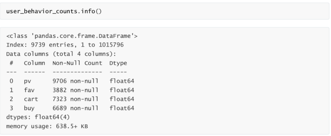
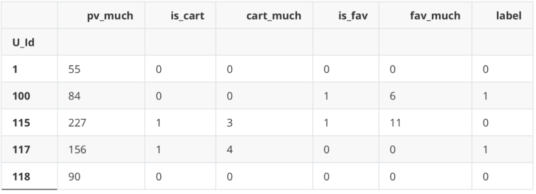
用户行为统计表

describe = df.loc[:,["U_Id","Be_type"]] ids = pd.DataFrame(np.zeros(len(set(list(df["U_Id"])))),index=set(list(df["U_Id"]))) pv_class=describe[describe["Be_type"]=="pv"].groupby("U_Id").count() pv_class.columns = ["pv"] buy_class=describe[describe["Be_type"]=="buy"].groupby("U_Id").count() buy_class.columns = ["buy"] fav_class=describe[describe["Be_type"]=="fav"].groupby("U_Id").count() fav_class.columns = ["fav"] cart_class=describe[describe["Be_type"]=="cart"].groupby("U_Id").count() cart_class.columns = ["cart"] user_behavior_counts=ids.join(pv_class).join(fav_class).join(cart_class).join(buy_class). iloc[:,1:] user_behavior_counts.head()

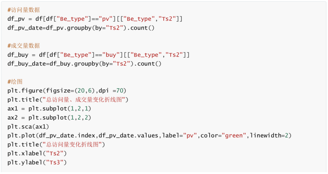
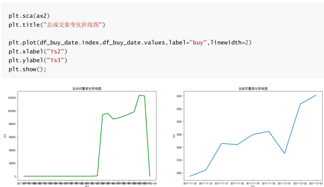
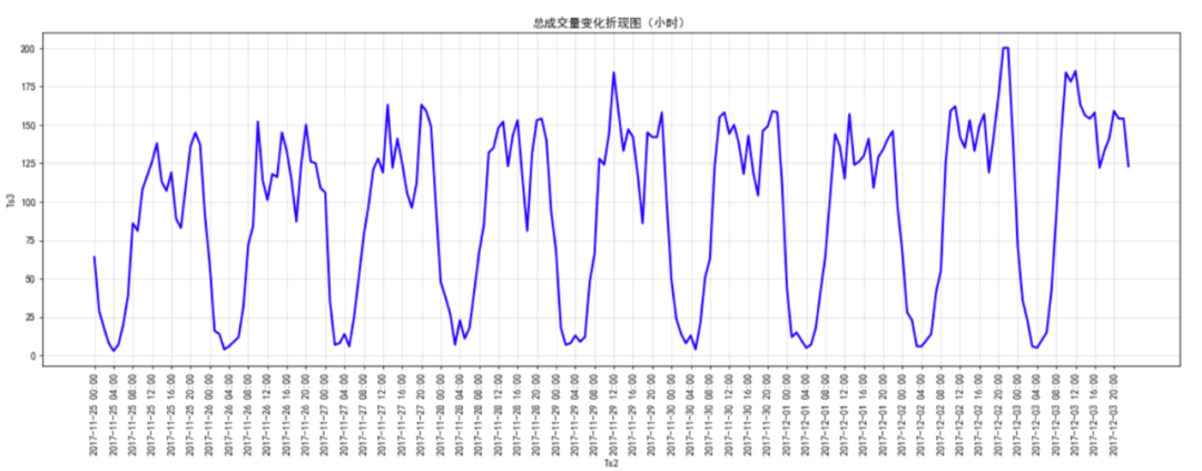
总访问量成交量时间变化分析(天) from matplotlib import font_manager # 解决坐标轴刻度负号乱码 # 解决负号'-'显示为方块的问题 plt.rcParams['axes.unicode_minus'] = False # 解决中文乱码问题 plt.rcParams['font.sans-serif'] = ['Simhei']

由总访问量、成交量时间变化分析知，从17年11月25日至17年12月1日访问量和成交量存在小幅波动，2017年12 月2日访问量和成交量均出现大幅上升，2日、3日两天保持高访问量和高成交量。此现象原因之一为12月2日和3 日为周末，同时考虑2日3日可能存在某些促销活动，可结合实际业务情况进行具体分析。(图中周五访问量有上升，但成交量出现下降，推测此现象可能与周末活动导致周五推迟成交有关。)

总访问量成交量时间变化分析(小时) # 数据准备 df_pv_timestamp=df[df["Be_type"]=="pv"][["Be_type","Ts1"]] df_pv_timestamp["Ts1"] = pd.to_datetime(df_pv_timestamp["Ts1"]) df_pv_timestamp=df_pv_timestamp.set_index("Ts1") df_pv_timestamp=df_pv_timestamp.resample("H").count()["Be_type"] df_pv_timestamp df_buy_timestamp=df[df["Be_type"]=="buy"][["Be_type","Ts1"]] df_buy_timestamp["Ts1"] = pd.to_datetime(df_buy_timestamp["Ts1"]) df_buy_timestamp=df_buy_timestamp.set_index("Ts1") df_buy_timestamp=df_buy_timestamp.resample("H").count()["Be_type"] df_buy_timestamp Ts1 2017-09-11 16:00:00 1 2017-09-11 17:00:00 0 2017-09-11 18:00:00 0 2017-09-11 19:00:00 0 2017-09-11 20:00:00 0 ... 2017-12-03 20:00:00 8587 2017-12-03 21:00:00 10413 2017-12-03 22:00:00 9862 2017-12-03 23:00:00 7226 2017-12-04 00:00:00 1 Freq: H, Name: Be_type, Length: 2001, dtype: int64 Ts1 2017-11-25 00:00:00 64 2017-11-25 01:00:00 29 2017-11-25 02:00:00 18 2017-11-25 03:00:00 8 2017-11-25 04:00:00 3 ... 2017-12-03 19:00:00 141 2017-12-03 20:00:00 159 2017-12-03 21:00:00 154 2017-12-03 22:00:00 154 2017-12-03 23:00:00 123 Freq: H, Name: Be_type, Length: 216, dtype: int64 #绘图 plt.figure(figsize=(20,6),dpi =70) x2= df_buy_timestamp.index plt.plot(range(len(x2)),df_buy_timestamp.values,label="成交量",color="blue",linewidth=2) plt.title("总成交量变化折现图(小时)") x2 = [i.strftime("%Y-%m-%d %H:%M") for i in x2] plt.xticks(range(len(x2))[::4],x2[::4],rotation=90) plt.xlabel("Ts2") plt.ylabel("Ts3") plt.grid(alpha=0.4);

特征工程

思路:不考虑时间窗口，只以用户的点击和收藏等行为来预测是否购买流程:以用户ID(U_Id)为分组键，将每位用户的点击、收藏、加购物车的行为统计出来，分别为

是否点击，点击次数;是否收藏，收藏次数;是否加购物车，加购物车次数

以此来预测最终是否购买

# 去掉时间戳 df = df[["U_Id", "T_Id", "C_Id", "Be_type"]] df

行为类型

U_Id 1 [1,1,1,1,1,1,1,1,1,1,1,1,1,1,1,... 100 [1,1,1,1,1,1,1,1,1,3,1,1,3,1,3,... 115 [1,1,1,1,1,1,1,1,1,1,1,1,1,1,3,... 117 [4,1,1,1,1,1,1,4,1,1,1,1,1,1,1,... 118 [1,1,1,1,1,1,1,1,1,1,1,1,1,1,1,... Name: Be_type1, dtype: object

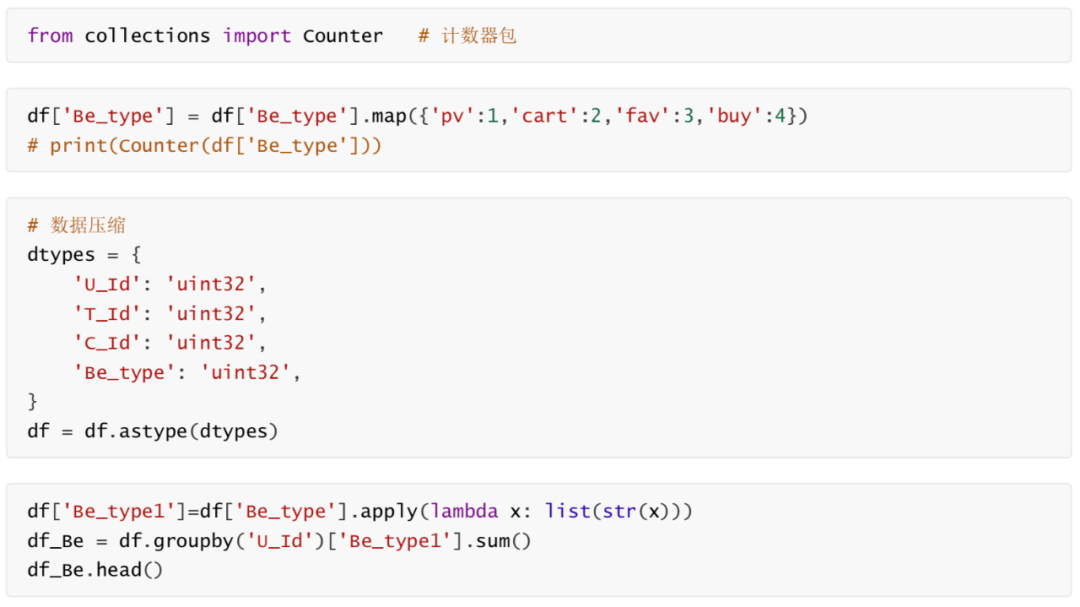
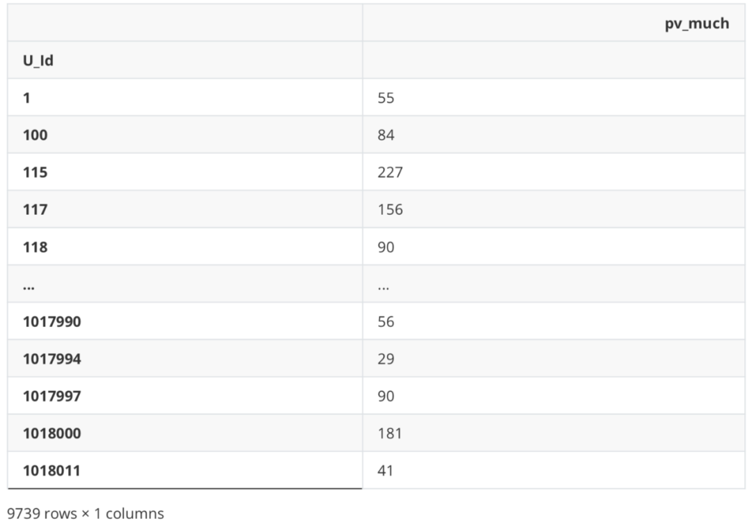
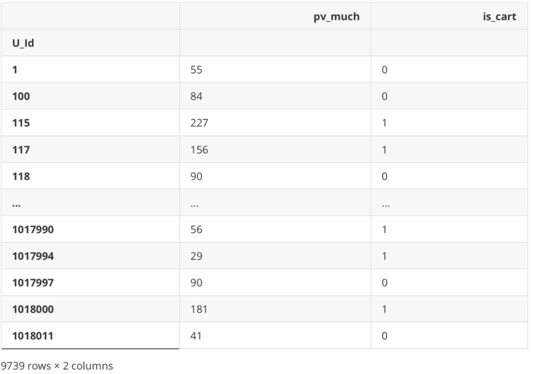
最后创建一个DataFrame用来存储等下计算出的用户行为。

df_new = pd.DataFrame() 点击次数 df_new['pv_much'] = df_Be.apply(lambda x: Counter(x)['1']) df_new

加购次数 #是否加购 df_new['is_cart'] = df_Be.apply(lambda x: 1 if '2' in x else 0) df_new

#加购了几次 df_new['cart_much'] = df_Be.apply(lambda x: 0 if '2' not in x else Counter(x)['2']) df_new

收藏次数 #是否收藏 df_new['is_fav'] = df_Be.apply(lambda x: 1 if '3' in x else 0) df_new

#收藏了几次 df_new['fav_much'] = df_Be.apply(lambda x: 0 if '3' not in x else Counter(x)['3']) df_new

相关分析 #部分数据 df_new.corr('spearman')

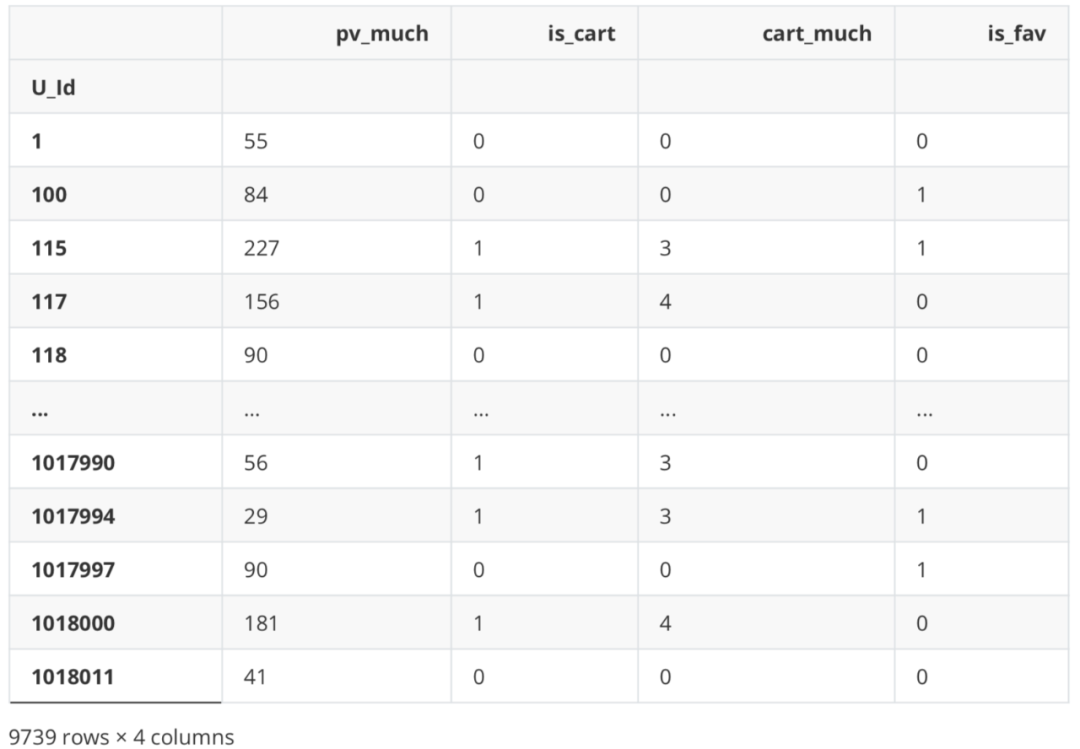
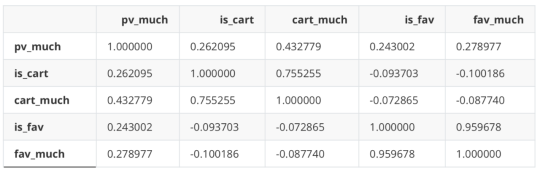
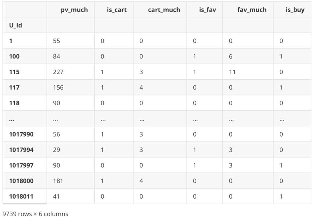
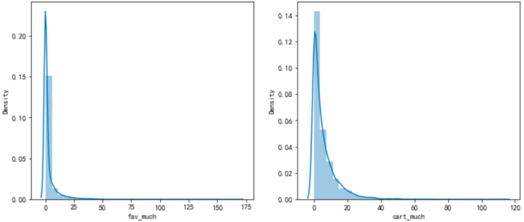
是否加购与加购次数、是否收藏与收藏次数之间存在一定相关性，但经验证剔除其中之一与纳入全部变量效果基本一致，故之后使用全部变量建模。

数据标签 import seaborn as sns #是否购买 df_new['is_buy'] = df_Be.apply(lambda x: 1 if '4' in x else 0) df_new

df_new.is_buy.value_counts() 1 6689 0 3050 Name: is_buy, dtype: int64 df_new['label'] = df_new['is_buy'] del df_new['is_buy'] df_new.head()

f,ax=plt.subplots(1,2,figsize=(12,5)) sns.set_palette(["#9b59b6","#3498db",]) #设置所有图的颜色，使用hls色彩空间 sns.distplot(df_new['fav_much'],bins=30,kde=True,label='123',ax=ax[0]); sns.distplot(df_new['cart_much'],bins=30,kde=True,label='12',ax=ax[1]); C:\Users\CDA\anaconda3\lib\site-packages\seaborn\distributions.py:2619: FutureWarning: `distplot` is a deprecated function and will be removed in a future version. Please adapt your code to use either `displot` (a figure-level function with similar flexibility) or `histplot` (an axes-level function for histograms). warnings.warn(msg, FutureWarning) C:\Users\CDA\anaconda3\lib\site-packages\seaborn\distributions.py:2619: FutureWarning: `distplot` is a deprecated function and will be removed in a future version. Please adapt your code to use either `displot` (a figure-level function with similar flexibility) or `histplot` (an axes-level function for histograms). warnings.warn(msg, FutureWarning)

建立模型

划分数据集

from sklearn.model_selection import train_test_split X = df_new.iloc[:,:-1] Y = df_new.iloc[:,-1] X.head() Y.head()

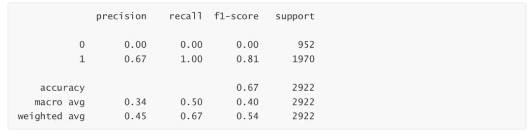
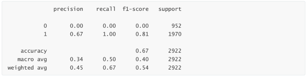
U_Id 10 100 1 115 0 117 1 118 0 Name: label, dtype: int64 Xtrain,Xtest,Ytrain,Ytest = train_test_split(X,Y,test_size= 0.3,random_state= 42) 逻辑回归

模型建立

from sklearn.linear_model import LogisticRegression LR_1 = LogisticRegression().fit(Xtrain,Ytrain) #简单测试 LR_1.score(Xtest,Ytest) 0.6741957563312799 模型评估 from sklearn import metrics from sklearn.metrics import classification_report from sklearn.metrics import auc,roc_curve #混淆矩阵 print(metrics.confusion_matrix(Ytest, LR_1.predict(Xtest))) [[ 0 952] [ 0 1970]] print(classification_report(Ytest,LR_1.predict(Xtest)))

D:\anaconda\lib\site-packages\sklearn\metrics\_classification.py:1308: UndefinedMetricWarning: Precision and F-score are ill-defined and being set to 0.0 in labels with no predicted samples. Use `zero_division` parameter to control this behavior. _warn_prf(average, modifier, msg_start, len(result)) D:\anaconda\lib\site-packages\sklearn\metrics\_classification.py:1308: UndefinedMetricWarning: Precision and F-score are ill-defined and being set to 0.0 in labels with no predicted samples. Use `zero_division` parameter to control this behavior. _warn_prf(average, modifier, msg_start, len(result)) D:\anaconda\lib\site-packages\sklearn\metrics\_classification.py:1308: UndefinedMetricWarning: Precision and F-score are ill-defined and being set to 0.0 in labels with no predicted samples. Use `zero_division` parameter to control this behavior. _warn_prf(average, modifier, msg_start, len(result)) fpr,tpr,threshold = roc_curve(Ytest,LR_1.predict_proba(Xtest)[:,1]) roc_auc = auc(fpr,tpr) print(roc_auc) 0.6379193682549162 随机森林

模型建立

from sklearn.ensemble import RandomForestClassifier rfc = RandomForestClassifier(n_estimators=200, max_depth=1) rfc.fit(Xtrain, Ytrain) RandomForestClassifier(max_depth=1, n_estimators=200) 模型评估 #混淆矩阵 print(metrics.confusion_matrix(Ytest, rfc.predict(Xtest))) [[ 0 952] [ 0 1970]] #分类报告 print(metrics.classification_report(Ytest, rfc.predict(Xtest)))

【本文地址】

Python 数据分析实战案例：用户行为预测

Python 数据分析实战案例：用户行为预测

今日新闻

推荐新闻