Arma模型预测时间序列的Matlab实现 |
您所在的位置:网站首页 › 参数预测模型 › Arma模型预测时间序列的Matlab实现 |
Arma模型预测时间序列的Matlab实现
|
Arma模型预测算法在两年之前有看过,当时没有太仔细看没能理解,最近结合网上几篇比较Nice 的关于ARMA && ARIMA算法的博客,对该算法有了进一步了解,将自己的理解进行整理。 1 概述Arma模型(自回归移动平均模型)是时间序列分析中常用的模型之一,它可以用于预测未来的时间序列值。Arma模型的核心思想是将时间序列看作是自回归和移动平均过程的组合。其中,自回归过程指的是时间序列值与其前一时刻值之间的关系;移动平均过程指的是时间序列值与其前一时刻的噪声误差之间的关系。 Arma模型可以表示为ARMA(p, q),其中p表示自回归项的阶数,q表示移动平均项的阶数。具体地,Arma模型可以写成如下形式: Y t = α 1 Y t − 1 + α 2 Y t − 2 + . . . + α p Y t − p + ϵ t + β 1 ϵ t − 1 + β 2 ϵ t − 2 + . . . + β q ϵ t − q Y_t=\alpha_1Y_{t-1}+\alpha_2Y_{t-2}+...+\alpha_pY_{t-p}+\epsilon_t+\beta_1\epsilon_{t-1}+\beta_2\epsilon_{t-2}+...+\beta_q\epsilon_{t-q} Yt=α1Yt−1+α2Yt−2+...+αpYt−p+ϵt+β1ϵt−1+β2ϵt−2+...+βqϵt−q 其中, Y t Y_t Yt表示时间序列在时刻t的值, ϵ t \epsilon_t ϵt表示在时刻t的噪声误差, α 1 \alpha_1 α1到 α p \alpha_p αp和 β 1 \beta_1 β1到 β q \beta_q βq分别表示自回归系数和移动平均系数。 Arma模型可以用于对时间序列进行预测和模拟,通常使用最小二乘法或极大似然法来估计模型参数。同时,Arma模型也可以通过对模型残差的分析来检验模型的拟合程度和合理性。 更加详细的理论可以参考这篇博文 2 算法主要流程 及 测试方案练习时没有使用真实时间序列,因为真实序列的周期项、趋势项中包含随机误差影响不可控,使不能够直观准确反应预测效果,这里使用模拟的时间序列进行测试,考虑到一个完整的序列是由周期项、半周期项、趋势项和随机误差组成,所以在模拟的时候对这些因素都进行了考虑;下面简单介绍下Arma的流程和测试的几种方案下得到的的结果。 主要流程 加载时间序列,检验序列是否平稳,常见的平稳性检验方法是adf和kpss检验,两种检验方法可能对同一序列有不同检验结果; %% matlab自带 ad1 = adftest(a4); % 1平稳 0非平稳 ad2 = kpsstest(a4); % 0 平稳 1 非平稳 如果检验显示序列非平稳,对序列进行差分直至序列达到平稳为止,一般差分1次就能满足平稳性要求; %% 对时间序列进行差分,并记录差分了几次 count = 0; arr1 = a4; while true arr21 = diff(arr1); count = count + 1; ad1 = adftest(arr21); % 1平稳 0非平稳 ad2 = kpsstest(arr21); % 0 平稳 1 非平稳 if ad1==1 && ad2 == 0 break end arr1 = arr21; end 模型定阶:定阶对预测结果还是比较重要的。参考博文,一般都是先看自相关(ACF) 和 偏相关(PACF)图,根据拖尾和截尾可以人工选择一个合适的阶数;如果人工选择比较困难,可以根据AIC、BIC准则定阶,具体理论可参考其他博文; % 自相关和偏相关图 figure(2) subplot(2,1,1) coll1 = autocorr(arr22); stem(coll1)%绘制经线图 title('自相关') subplot(2,1,2) coll2 = parcorr(arr22); stem(coll2)%绘制经线图 title('偏相关') % Aic准则 value = aic(AmMode); 序列预测:在预测的时候要考虑序列是否进行过差分(diff),因为非平稳序列差分后进行预测的,预测结果也是差分后的结果,此时要对序列还原 才能得到原序列的预测; % 预测 aaa = predict(model, arr2, ntest); %利用arr2去向后预测 % 序列还原 hhh = cumsum([a4(1);difvalue]);%还原差分几种方案 由于时间序列是模拟的,所以可以控制生成周期、周期+趋势、周期+趋势+噪声、周期+噪声这几个类型的时间序列,根据对不同序列的预测效果,可以看到ARMA对不同序列的适用性; a. 纯周期序列 对比发现,周期序列的预测效果较好; 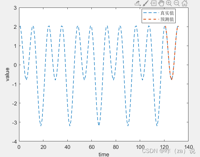 预测结果
预测结果
b. 纯周期+噪声 这种情况下,预测效果就没有特别好了,所以在一些情况下可以对序列进行滤波后再进行预测;  预测结果
预测结果
c. 纯周期+趋势+噪声 这种情况预测效果不太好; 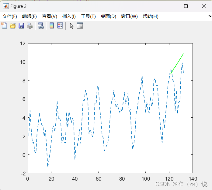 预测结果
预测结果
d. 周期+趋势 没有噪声时这个预测结果也是可以的。 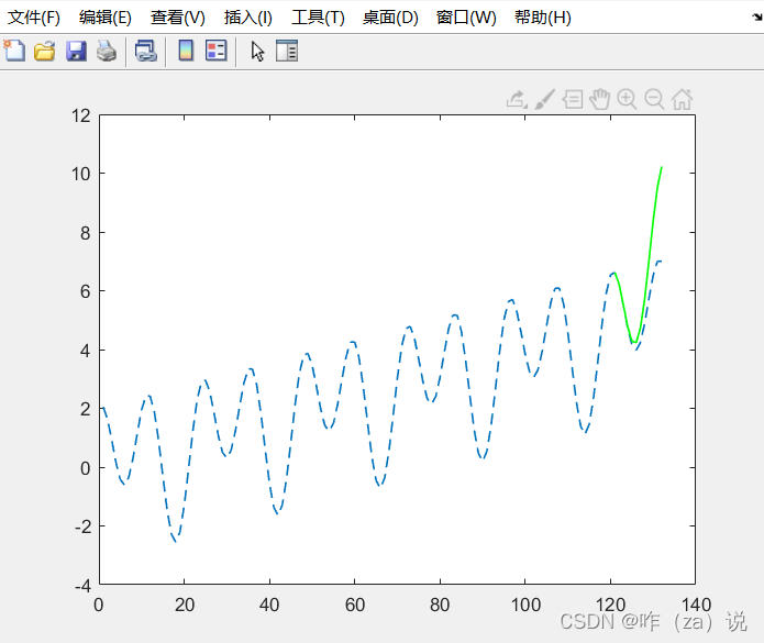 预测结果
预测结果
所以,经过对比能看出,噪声对预测结果影响较大,没有噪声的情况下,ARMA/ARIMA的预测效果大概有一定可信性。 3 Matlab代码运行程序 %% 主程序 %% 1 生成模拟信号 clear; n = 132; % 模拟11年的数据,用10年的数据作为训练值 ntest = 12; %用最后1年数据作为预测比对值 x = 1:n; % 周期信号 a1 = cos(2*pi*x/12) + 0.6 * sin(2*pi*x/24); figure(1) subplot(2,2,1) plot(x,a1); title('a1 周期信号') % 趋势信号 subplot(2,2,2); x2=0.14; a2 = mapminmax(x2 * x,0,1); plot(x,a2); title('a2 趋势信号') % 随机信号(0-1的随机值) subplot(2,2,3) a3 = rand(1,n); plot(x,a3); title('a3 随机信号') % 三种信号叠加 生成模拟信号 subplot(2,2,4) % %a41 = 2 .* a1; % 1 只有周期项 %a41 = 2 .* a1 + 3.2 * a3; % 2 周期 + 随机 %a41 = 2 .* a1 + 5 * a2 + 3.2 * a3; % 3 周期 + 趋势 + 随机 a41= 2 .* a1 + 5 * a2; plot(x,a41); title('a4 叠加序列') %% 平稳检验 a4 = a41(1:n-ntest); ad1 = adftest(a4); % 1平稳 0非平稳 ad2 = kpsstest(a4); % 0 平稳 1 非平稳 if (ad1 == 1 && ad2 == 0) % 平稳 type = 3; else % 非平稳 type = 4; end %% type 可以自行输入 switch type case 1 datas = 0; case 2 datas = 0; case 3 % 平稳序列 arma datas = function_arma(a4,ntest); %% 绘图 figure(3) plot(1:n,a41,'--','LineWidth',1) hold on plot((n-ntest)+1:n,datas((n-ntest)+1:n),'--','LineWidth',1.5) hold on xlabel('time') ylabel('value') legend('真实值','预测值') case 4 % 非平稳序列 arima [Y,lower,upper] = function_arima(a4,ntest); figure(3); plot(1:n,a41,'--','LineWidth',1) hold on; plot( (n - ntest+1 : n), Y, 'g', 'LineWidth', 1); end %% 平稳平稳 arma预测 %% a4训练数据 ntest预测长度 function data = function_arma(a4,ntest) %自相关、偏自相关 figure(2) subplot(2,1,1) coll1 = autocorr(a4); stem(coll1)%绘制经线图 title('自相关') subplot(2,1,2) coll2 = parcorr(a4); stem(coll2)%绘制经线图 title('偏相关') % count2 = length(a4); limvalue = round(count2 / 10); if(limvalue > 10) limvalue = 10; end % 计算最佳的p 和 q [bestp,bestq] = Select_Order_arma(a4, limvalue, limvalue); % 得到最佳模型 xa4 = iddata(a4'); model = armax(xa4,[bestp,bestq]); % 开始预测,获取预测数据 arr1 = [a4';zeros(ntest,1)]; arr2 = iddata(arr1); arr3=predict(model, arr2, ntest); %利用arr2去向后预测 arr4 = get(arr3); dataPre = arr4.OutputData{1,1}(length(a4)+1:length(a4)+ntest); data=[a4';dataPre]; % 获取训练结果加预测结果 end %% Arma找最优阶数 function [p1,p2] = Select_Order_arma(x2, limp, limq) array = zeros(limp, limq); x = iddata(x2'); for i =1:limp for j = 1:limq AmMode = armax(x,[i,j]); value = aic(AmMode); array(i,j) = value; end end [p1,p2]=find(array==min(min(array))); end %% ARIMA %% 非平稳序列 function [preData,LLL,UUU] = function_arima(a4,ntest) % 差分 count = 0; arr1 = a4; while true arr21 = diff(arr1); count = count + 1; ad1 = adftest(arr21); % 1平稳 0非平稳 ad2 = kpsstest(arr21); % 0 平稳 1 非平稳 if ad1==1 && ad2 == 0 break end arr1 = arr21; end arr22 = arr21'; % 自相关 figure(2) subplot(2,1,1) coll1 = autocorr(arr22); stem(coll1)%绘制经线图 title('自相关') subplot(2,1,2) coll2 = parcorr(arr22); stem(coll2)%绘制经线图 title('偏相关') % 此时是平稳的 count2 = length(arr22); limvalue = round(count2 / 10); if(limvalue > 3) limvalue = 3; end % 计算最佳的p 和 q [bestp,bestq] = Select_Order_arima(arr22, limvalue, limvalue, count); modelo = arima(bestp,count,bestq); md1 = estimate(modelo, arr22); [Y, YMSE] = forecast(md1, ntest, 'Y0', arr22); lower = Y - 1.96*sqrt(YMSE); %95置信区间下限 upper = Y + 1.96*sqrt(YMSE); difvalue = [arr22;Y]; %差分序列 difvalueL = [arr22;lower]; difvalueU = [arr22;upper]; count2 = length(a4); if(count >=1) hhh = cumsum([a4(1);difvalue]);%还原差分值 LLL1 = cumsum([a4(count2);difvalueL]); UUU1 = cumsum([a4(count2);difvalueU]); end preData = hhh(length(a4)+1 : (length(a4) + ntest)); LLL = LLL1(length(a4)+1 : (length(a4) + ntest)); UUU = UUU1(length(a4)+1 : (length(a4) + ntest)); end %% Arima找最优阶数 function [best_p,best_q] = Select_Order_arima(data, pmax, qmax, d) min_aic = Inf; min_bic = Inf; best_p = 0; best_q = 0; for p=0:pmax for q=0:qmax model = arima(p,d,q); try [fit,~,logL]=estimate(model,data); [aic, bic] = aicbic(logL, p + q + 1, length(data)); catch continue end if aic |
【本文地址】
今日新闻 |
推荐新闻 |