[机器学习 |
您所在的位置:网站首页 › 决策树概念图 › [机器学习 |
[机器学习
|
决策树学习与总结 (ID3, C4.5, C5.0, CART)
1. 什么是决策树2. 决策树介绍3. ID3 算法信息熵信息增益缺点
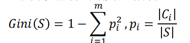
4. C4.5算法5. C5.0算法6. CART算法基尼指数 Gini指标
7. 连续属性离散化8. 过拟合的解决方案9. 例子1 - 脊椎动物分类10. 例子21. 准备数据及读取2. 决策树的特征向量化3. 决策树训练4. 决策树可视化5 预测结果6. Module persistence1) 用Python有的pickle对我们训练好的模型保存2) 用joblib’s保持如果你的模型里有大量的 numpy arrays的话
7. 自己算验证熵的结果8. 如果你用基尼指数, 也就是CART算法9. 自己算验证基尼指数的结果10. 把数据集全部改成数字不用DictVectorizer做向量化
11. 例子 -基于Iris数据集的训练12. 特征的重要性计算可能遇到问题
1. 什么是决策树
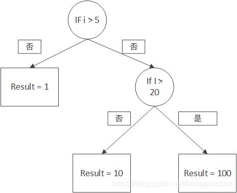
决策树是什么,我们来“决策树”这个词进行分词,那么就会是决策/树。大家不妨思考一下,重点是决策还是树呢?其实啊,决策树的关键点在树上。 我们平时写代码的那一串一串的If Else其实就是决策树的思想了。看下面的图是不是觉得很熟悉呢?
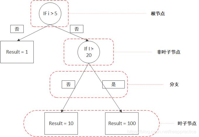
决策树之所以叫决策树,就是因为它的结构是树形状的,如果你之前没了解过树这种数据结构,那么你至少要知道以下几个名词是什么意思。 根节点:最顶部的那个节点叶子节点:每条路径最末尾的那个节点,也就是最外层的节点非叶子节点:一些条件的节点,下面会有更多分支,也叫做分支节点分支:也就是分叉
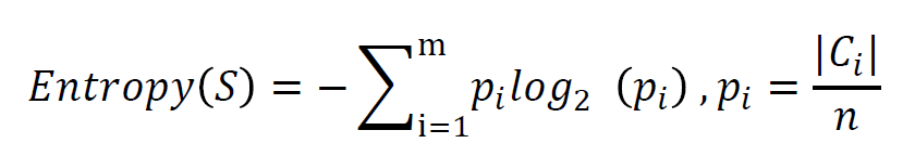
不理解信息熵的可以看这篇博客[机器学习-概念篇]彻底搞懂信息量,熵、相对熵、交叉熵 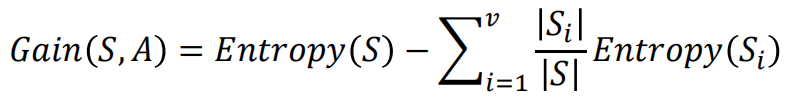 脊椎动物分类训练样本集 脊椎动物分类训练样本集 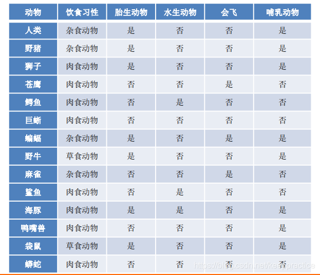 共有14个样本,其中8个正例,6个反例,设此样本集为 S,则分裂前的熵值为 共有14个样本,其中8个正例,6个反例,设此样本集为 S,则分裂前的熵值为 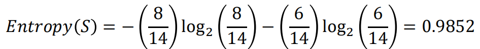 脊椎动物训练样本集以“饮食习性”作为分支属性的分裂情况 脊椎动物训练样本集以“饮食习性”作为分支属性的分裂情况 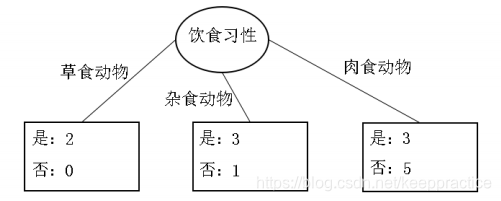 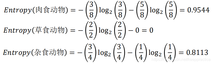 设“饮食习性”属性为Y,由此可以计算得出,作为分支属性进行分裂之后的 信息增益为 设“饮食习性”属性为Y,由此可以计算得出,作为分支属性进行分裂之后的 信息增益为 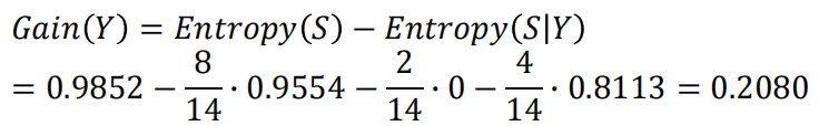 同理, 计算可得,以“胎生动物”“水生动物”“会飞”作为分支属性时的信息 增益分别为0.6893、0.0454、0.0454 由此可知“胎生动物”作为分支属性时能获得最大的信息增益,即具有最强的区分样本的能力,所以在此选择使用“胎生动物”作为分支属性对根结点进行划分 由根结点通过计算信息增益选取合适的属性进行分裂,若新生成的结点的分类属性不唯一,则对新生的结点继续进行分裂,不断重复此步骤,直至所有样本属于同 一类,或者达到要求的分类条件为止
缺点
4. C4.5算法 同理, 计算可得,以“胎生动物”“水生动物”“会飞”作为分支属性时的信息 增益分别为0.6893、0.0454、0.0454 由此可知“胎生动物”作为分支属性时能获得最大的信息增益,即具有最强的区分样本的能力,所以在此选择使用“胎生动物”作为分支属性对根结点进行划分 由根结点通过计算信息增益选取合适的属性进行分裂,若新生成的结点的分类属性不唯一,则对新生的结点继续进行分裂,不断重复此步骤,直至所有样本属于同 一类,或者达到要求的分类条件为止
缺点
4. C4.5算法
C4.5算法总体思路与ID3类似,都是通过构造决策树进行分类,其区别在于分支的处理,在分支属性的选取上,ID3算法使用信息增益作为度量,而C4.5算法引入了信息增益率作为度量 CART算法在分支处理中分支属性的度量指标 如果是连续的数值型是如年龄,我们一般把它离散化,如离散化为幼年,中年,老年 因为你不可能让把每个年龄都分成一个特征,那样会很多,也没必要。 8. 过拟合的解决方案 一方面要注意数据训练集的质量,选取具有代表性样本的训练样本集要避免决策树过度增长,通过限制树的深度来减少数据中的噪声对于决策树构建的影响,一般可以采取剪枝的方法剪枝包括预剪枝和后剪枝两类 预剪枝的思路是提前终止决策树的增长,在形成完全拟合训练样本集的决 策树之前就停止树的增长,避免决策树规模过大而产生过拟合 后剪枝策略先让决策树完全生长,之后针对子树进行判断,用叶子结点或者子树中最常用的分支替换子树,以此方式不断改进决策树,直至无法改进为止 9. 例子1 - 脊椎动物分类脊椎动物分类训练样本集 test.csv 文件, 做了下面的变换 是:0, 否 : 1 ,杂食动物 : omnivorous animal, 肉食动物:carnivorous animals, : 草食动物, herbivore omnivorous animal, 0, 1, 1, 0 omnivorous animal, 0, 1, 1, 0 carnivorous animals, 0, 1, 1, 0 carnivorous animals, 1, 1, 0, 1 carnivorous animals, 1, 0, 1, 1 carnivorous animals, 1, 1, 1, 1 omnivorous animal, 0, 1, 0, 0 herbivore, 0, 1, 1, 0 omnivorous animal, 1, 1, 0, 1 carnivorous animals, 1, 0, 1, 1 carnivorous animals, 0, 0, 1, 0 carnivorous animals, 1, 1, 1, 0 herbivore, 0, 1, 1, 0 carnivorous animals, 1, 1, 1, 1代码 import pandas as pd import sklearn as sklearn from sklearn.feature_extraction import DictVectorizer from sklearn import tree import pydotplus from sklearn.externals.six import StringIO # pandas 读取 csv 文件,header = None 表示不将首行作为列 data = pd.read_csv('data/test.csv', header=None) # 指定列 data.columns = ['Diet Habits', 'viviparous animal', 'Aquatic animals', 'Can fly','mammal'] # sparse=False意思是不产生稀疏矩阵 vec = sklearn.feature_extraction.DictVectorizer(sparse=False) # 先用 pandas 对每行生成字典,然后进行向量化 feature = data[['Diet Habits', 'viviparous animal', 'Aquatic animals']] X_train = vec.fit_transform(feature.to_dict(orient='record')) # 打印各个变量 print('show feature\n', feature) print('show vector\n', X_train) print('show vector name\n', vec.get_feature_names()) print('show vector name\n', vec.vocabulary_) Y_train = data['mammal'] clf = tree.DecisionTreeClassifier(criterion='entropy') clf.fit(X_train, Y_train) dot_data = StringIO() tree.export_graphviz(clf,feature_names=vec.get_feature_names(),out_file=dot_data) graph = pydotplus.graph_from_dot_data(dot_data.getvalue()) graph.write_pdf("test.pdf") show feature Diet Habits viviparous animal Aquatic animals 0 omnivorous animal 0 1 1 omnivorous animal 0 1 2 carnivorous animals 0 1 3 carnivorous animals 1 1 4 carnivorous animals 1 0 5 carnivorous animals 1 1 6 omnivorous animal 0 1 7 herbivore 0 1 8 omnivorous animal 1 1 9 carnivorous animals 1 0 10 carnivorous animals 0 0 11 carnivorous animals 1 1 12 herbivore 0 1 13 carnivorous animals 1 1 show vector [[1. 0. 0. 1. 0.] [1. 0. 0. 1. 0.] [1. 1. 0. 0. 0.] [1. 1. 0. 0. 1.] [0. 1. 0. 0. 1.] [1. 1. 0. 0. 1.] [1. 0. 0. 1. 0.] [1. 0. 1. 0. 0.] [1. 0. 0. 1. 1.] [0. 1. 0. 0. 1.] [0. 1. 0. 0. 0.] [1. 1. 0. 0. 1.] [1. 0. 1. 0. 0.] [1. 1. 0. 0. 1.]] show vector name ['Aquatic animals', 'Diet Habits=carnivorous animals', 'Diet Habits=herbivore', 'Diet Habits=omnivorous animal', 'viviparous animal'] show vector name {'Diet Habits=omnivorous animal': 3, 'viviparous animal': 4, 'Aquatic animals': 0, 'Diet Habits=carnivorous animals': 1, 'Diet Habits=herbivore': 2}
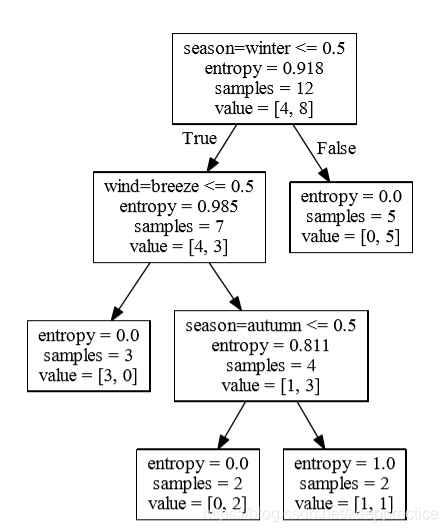
安装panda 和 scikit-learn 如果你没有安装的话 conda install pandas conda install scikit-learn 1. 准备数据及读取 季节时间已过 8 点风力情况要不要赖床springnobreezeyeswinternono windyesautumnyesbreezeyeswinternono windyessummernobreezeyeswinteryesbreezeyeswinternogaleyeswinternono windyesspringyesno windnosummeryesgalenosummernogalenoautumnyesbreezeno spring,no,breeze,1 winter,no,no wind,1 autumn,yes,breeze,1 winter,no,no wind,1 summer,no,breeze,1 winter,yes,breeze,1 winter,no,gale,1 winter,no,no wind,1 spring,yes,no wind,0 summer,yes,gale,0 summer,no,gale,0 autumn,yes,breeze,0 2. 决策树的特征向量化sklearn的DictVectorizer能对字典进行向量化。什么叫向量化呢?比如说你有季节这个属性有[春,夏,秋,冬]四个可选值,那么如果是春季,就可以用[1,0,0,0]表示,夏季就可以用[0,1,0,0]表示。不过在调用DictVectorizer它会将这些属性打乱,不会按照我们的思路来运行,但我们也可以一个方法查看,我们看看代码就明白了 通过DictVectorizer,我们就能够把字符型的数据,转化成0 1的矩阵,方便后面进行运算。额外说一句,这种转换方式其实就是one-hot编码。 import pandas as pd import sklearn as sklearn from sklearn.feature_extraction import DictVectorizer from sklearn import tree # pandas 读取 csv 文件,header = None 表示不将首行作为列 data = pd.read_csv('data/laic.csv', header=None) # 指定列 data.columns = ['season', 'after 8', 'wind', 'lay bed'] # sparse=False意思是不产生稀疏矩阵 vec = DictVectorizer(sparse=False) # 先用 pandas 对每行生成字典,然后进行向量化 feature = data[['season', 'after 8', 'wind']] X_train = vec.fit_transform(feature.to_dict(orient='record')) # 打印各个变量 print('show feature\n', feature) print('show vector\n', X_train) print('show vector name\n', vec.get_feature_names()) print('show vector name\n', vec.vocabulary_)执行结果 show feature season after 8 wind 0 spring no breeze 1 winter no no wind 2 autumn yes breeze 3 winter no no wind 4 summer no breeze 5 winter yes breeze 6 winter no gale 7 winter no no wind 8 spring yes no wind 9 summer yes gale 10 summer no gale 11 autumn yes breeze show vector [[1. 0. 0. 1. 0. 0. 1. 0. 0.] [1. 0. 0. 0. 0. 1. 0. 0. 1.] [0. 1. 1. 0. 0. 0. 1. 0. 0.] [1. 0. 0. 0. 0. 1. 0. 0. 1.] [1. 0. 0. 0. 1. 0. 1. 0. 0.] [0. 1. 0. 0. 0. 1. 1. 0. 0.] [1. 0. 0. 0. 0. 1. 0. 1. 0.] [1. 0. 0. 0. 0. 1. 0. 0. 1.] [0. 1. 0. 1. 0. 0. 0. 0. 1.] [0. 1. 0. 0. 1. 0. 0. 1. 0.] [1. 0. 0. 0. 1. 0. 0. 1. 0.] [0. 1. 1. 0. 0. 0. 1. 0. 0.]] show vector name ['after 8=no', 'after 8=yes', 'season=autumn', 'season=spring', 'season=summer', 'season=winter', 'wind=breeze', 'wind=gale', 'wind=no wind'] show vector name {'season=spring': 3, 'after 8=no': 0, 'wind=breeze': 6, 'season=winter': 5, 'wind=no wind': 8, 'season=autumn': 2, 'after 8=yes': 1, 'season=summer': 4, 'wind=gale': 7} 3. 决策树训练 Y_train = data['lay bed'] clf = tree.DecisionTreeClassifier(criterion='entropy') clf.fit(X_train, Y_train) 4. 决策树可视化当完成一棵树的训练的时候,我们也可以让它可视化展示出来,不过sklearn没有提供这种功能,它仅仅能够让训练的模型保存到dot文件中。但我们可以借助其他工具让模型可视化,先看保存到dot的代码: with open("out.dot", 'w') as f : f = tree.export_graphviz(clf, out_file = f, feature_names = vec.get_feature_names()) 5 预测结果 result = clf.predict([[1., 0., 0. ,1. , 0. , 0. , 1. , 0. , 0.]]) print(result) [1]然后可以执行下面命令生成一个out.pdf dot out.dot -T pdf -o out.pdf
两种方式保持我们的模型 参考Sklearn 官网 1) 用Python有的pickle对我们训练好的模型保存 import pickle with open('decisive_tree_module.txt', 'wb') as f: pickle.dump(clf, f) with open('decisive_tree_module.txt', 'rb') as f: clf2 = pickle.load(f) #s = pickle.dumps(clf) #clf2 = pickle.loads(s) predict2 = clf2.predict([[1., 0., 0. ,1. , 0. , 0. , 1. , 0. , 0.]]) print('Predict result via loading pickle saved module :', predict2) Predict result via loading pickle saved module : [1] 2) 用joblib’s保持如果你的模型里有大量的 numpy arrays的话 from joblib import dump, load dump(clf, 'jdecisive_tree_module.joblib') clf3 = load('jdecisive_tree_module.joblib') predict3 = clf3.predict([[1., 0., 0. ,1. , 0. , 0. , 1. , 0. , 0.]]) print('Predict result via loading joblib saved module :', predict3) Predict result via loading joblib saved module : [1] 7. 自己算验证熵的结果 import math root_node_entropy = -(8/12)*(math.log(8/12, 2)) - (4/12)*(math.log(4/12, 2)) node1_left = (-(3/7)*(math.log(3/7, 2)) - (4/7)*(math.log(4/7,2))) #node1_right = (-(5/5)*(math.log(5/5, 2)) - (0/5)*(math.log(0/5,2))) node1_right = (-(5/5)*(0) - 0) #node2_left = -(3/3)*(math.log(3/3, 2)) - (0/3)*(math.log(0/3, 2)) node2_left = -(3/3)*(0) - 0 node2_right = -(3/4)*(math.log(3/4, 2)) - (1/4)*(math.log(1/4, 2)) print('Entropy of season=winter ', root_node_entropy) print('Entropy of wind=breeze ', node1_left) print('Entropy of wind=breeze ', node1_right) print('Entropy of node2_left', node2_left) print('Entropy of node2_right', node2_right) Entropy of season=winter 0.9182958340544896 Entropy of wind=breeze 0.9852281360342516 Entropy of wind=breeze -0.0 Entropy of node2_left -0.0 Entropy of node2_right 0.8112781244591328 8. 如果你用基尼指数, 也就是CART算法只需要把entropy 改成 gini就可以了 clf = tree.DecisionTreeClassifier(criterion='gini')
spring :1 , summer : 2, spring : 3 , winter : 4 时间已过 8 点-no : 0 时间已过 8 点-yes :1 breeze : 1 , no wind : 2 , gale :3 laic1.csv 文件 1,0,1,1 4,0,2,1 3,1,1,1 4,0,2,1 2,0,1,1 4,1,1,1 4,0,3,1 4,0,2,1 1,1,2,0 2,1,3,0 2,0,3,0 3,1,1,0代码 import pandas as pd from sklearn import tree data = pd.read_csv('data/laic1.csv', header=None) # 指定列 data.columns = ['season', 'after 8', 'wind', 'lay bed'] X_train = data[['season', 'after 8', 'wind']] Y_train = data['lay bed'] clf = tree.DecisionTreeClassifier(criterion='entropy') clf.fit(X_train, Y_train) with open("out1.dot", 'w') as f : f = tree.export_graphviz(clf, out_file = f, feature_names =['season', 'after 8', 'wind'])结果, 可以看到决策树图其实都一样的。 数据集如下
这棵树总的不纯减少量为4.262+1.281+0.883=6.426 经过归一化后,各特征的重要性分别如下: f1_importance = 4.262/6.426=0.663 f2_importance = 0 f3_importance = 1.281/6.426=0.2 f4_importance = 0.883/6.426=0.137 使用代码跑出来的特征重要性如下 from sklearn.tree import DecisionTreeClassifier train_df = pd.DataFrame( [[1, 1, 1, 1, 0], [1, 1, 1, 2, 0], [2, 1, 1, 1, 1], [3, 2, 1, 1, 1], [3, 3, 2, 1, 1], [3, 3, 2, 2, 0], [2, 3, 2, 2, 1], [1, 2, 1, 1, 0], [1, 3, 2, 1, 1], [3, 2, 2, 1, 1], [1, 2, 2, 2, 1], [2, 2, 1, 2, 1], [2, 1, 2, 1, 1], [3, 2, 1, 2, 0], ], columns=['f1', 'f2', 'f3', 'f4', 'label']) X, y = train_df[['f1', 'f2', 'f3', 'f4']].values, train_df['label'] clf = DecisionTreeClassifier(criterion='gini') clf.fit(X,y) print(clf.feature_importances_) # 特征重要性 [0.66296296 0. 0.2 0.13703704] 可能遇到问题如果你这个graphvis 的问题 (GraphViz’s executables not found), 可以根据下面这个link解决它 https://blog.csdn.net/qq_40304090/article/details/88594813 |
 举例来说,如果有一个大小为10的布尔值样本集S𝑏,其中有6个真值、4个 假值,那么该布尔型样本分类的熵为:
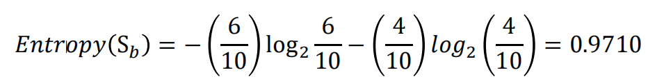
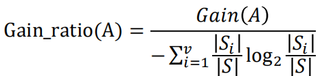 由信息增益率公式中可见,当𝑣比较大时,信息增益率会明显降低,从而在一定程度上能够解决ID3算法存在的往往选择取值较多的分支属性的问题 在前面例子中,假设选择“饮食习性”作为分支属性,其信息增益率为
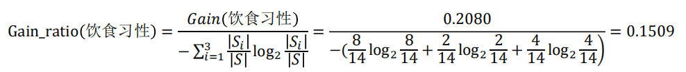
 在前面例子中,假设选择“会飞”作为分支属性,其Gini指标为
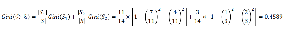

 预测结果
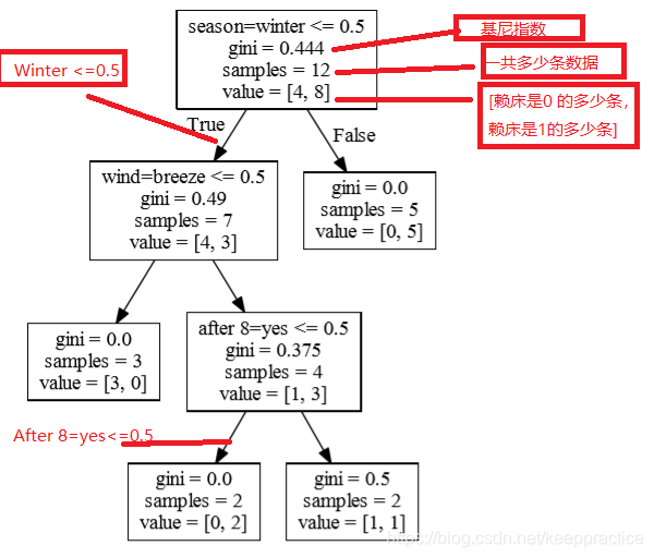
预测结果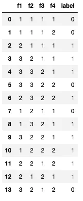 构建决策树,使用gini系数作为切割参数,决策数为cart树。生成的树结构如下
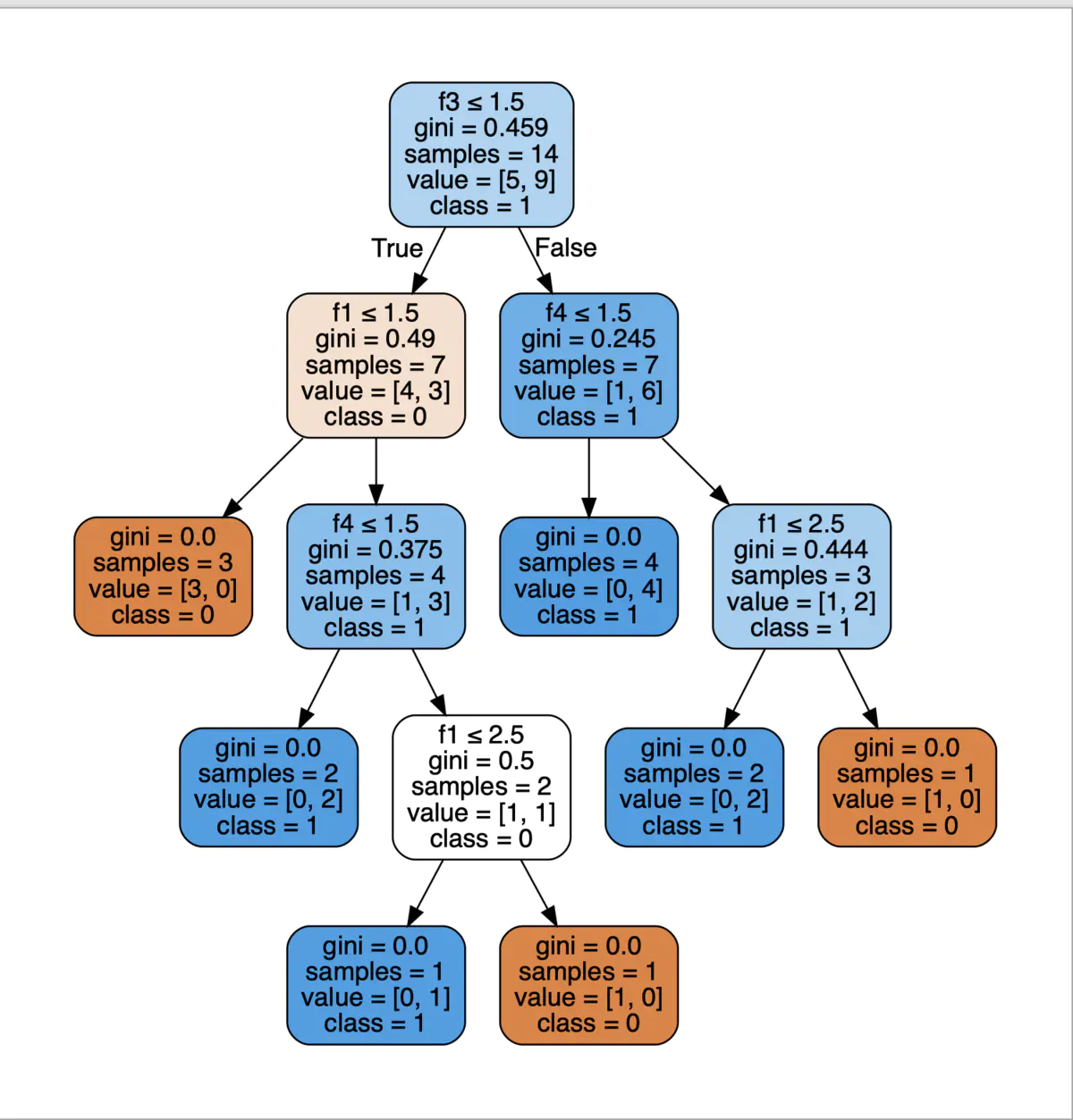 计算个特征的重要性 f1 = 0.497 - 0.3754 + 0.52 + 0.4443 = 4.262 f2 = 0 f3 = 0.45914 - 0.497 - 0.2457 = 1.281 f4 = 0.2457 - 0.4443 + 0.3754 - 0.5*2 = 0.883
【本文地址】
今日新闻 |
推荐新闻 |