定义：光束在垂直于光轴平面上的电场可由高斯方程表示，有时还会有附加的抛物线型相位曲线。    尤其是在激光物理中，激光光束通常为高斯光束，是以数学家和物理学家Johann Carl Friedrich Gauß命名。这时功率为P的光束光强的横断面可由高斯方程表示：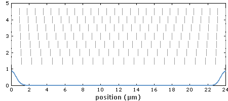 

这里光束半径w(z)为光强降为峰值的1/e2 (≈ 13.5%)时距光轴的距离。孔径半径为w时可以透射约86.5%的光功率。如果孔径半径为1.5w或者2w，传输比例分别提高到 98.9%和99.97%。 除了强度可以采用高斯方程描述，高斯光束的横向相位曲线可由最多二阶多项式来描述。在一个方向上相位的线性变化可由一个倾角描述，相位的二阶变化则与光束的发散和会聚相关。 

         高斯光束的传输 通常在傍轴近似适用的情况下将光束看做高斯光束，即光束发散角比较小。这一近似下，传播方程中的二阶导数项可以忽略，只得到一阶微分方程。并且采用这种近似时，高斯光束在自由空间中传播仍然保持高斯型，其参数会发生一些变化。一束单色光束，波长为 λ，在z轴传播时，电场的复振幅为： 

最大幅值为|E0|，束腰处的光束半径为 w0，波数 k = 2π / λ，zR为瑞利长度，波前的曲率半径为R(z)。震荡的实数电场可以通过乘以相位因子exp(i 2π c t / λ) 并且取实部得到。 

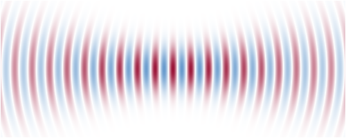图1：高斯光束焦点处的电场分布。这时光束半径比波长稍大，光速发散角很大。根据以上方程，场由左侧向右侧移动。 在传播方向上的光束半径变化为： 

其中瑞利长度为： 

决定了在多长距离范围内光束不会发散很严重的传播。（之前通常采用共焦长b描述，它是瑞利长度的二倍。）准直光束（光束半径接近于常数）的瑞利长度与传播距离相比比较大。 

 图2：高斯光束的光束半径变化（蓝色曲线）。两条竖线代表瑞利长度，虚线表明远离束腰的渐变变化情况。 以上方程中 z = 0对应于束腰或者焦点，在该点光束半径是最小的，相位曲线是平坦的。波前曲率半径为R的演化遵循方程： 

 在透明介质中传播时，λ是介质中的波长（非真空波长）。上面采用的其它参数和方程都不用改变，这时假设了介质是各向同性、均匀和无损耗的。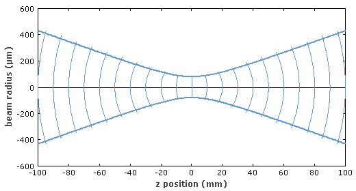 

图3：具有弯曲波前的高斯光束。在接近于焦点和远离焦点时曲率都很小。 电场中的反正切项对应的是古依相移，对于光学谐振腔的谐振频率非常重要。 远场的光束发散角为： 

 表明束腰半径越小，波长越长，则远离束腰后光束的发散越强。高斯光束的光束参数乘积（束腰半径与远场发散角的乘积）等于 λ/π，只与波长有关。如果激光光束的光束质量是非理想的，该值会更大。 傍轴近似需要焦点处光束半径比波长大。这表明这时光束发散角不会很大，并且瑞利长度远大于光束半径。紧聚焦光束一般不能很好的满足傍轴近似，这时需要更加复杂的方法来计算光束传播情况。 

复数参数 在z处高斯光束的状态可以由一个复数q表征： 

 这样复电场可写为： 

传输一定距离可以简单的表示为该距离上q参数的增加。当高斯光束通过一个曲面镜或者透镜时， q参数变化可由ABCD矩阵表示： 

像散光束 在两垂直的横平面方向上，写为x和y方向，高斯光束的半径和发散角可能不同。上面给出的方程可分别用来描述每一方向上光束半径的变化。如果两个方向上的焦点位置不重合，就称该光束是像散的。 

高斯光束和谐振腔模式 如果谐振腔是稳定的，谐振腔中的光学介质是各项同性的，介质表面要么是平坦的或者是抛物线形状的，那么光学谐振腔横向的最低阶模式（TEM00或者横向基模）就是高斯模。因此，只辐射横向基模的激光器辐射的光束接近于高斯型。而任何偏离之前描述的条件，例如，增益介质中存在热透镜效应等，都会使光束为非高斯型，同时还会激发多个纵模。更高阶纵模可由厄米-高斯方程或者拉盖尔-高斯方程来描述。任意情况下，与高斯谱型的偏离都可以由 M2因子定量表示。高斯光束具有最高的光束质量，对应的光束参量乘积最小，并且对应的M2 = 1。 光纤的基模并不严格为高斯型，但是形状与高斯型差别不是很大。因此，采用合适的光学元件，高斯光束可以有效进入单模光纤中（80%或更大）。 

高斯光束的重要性 高斯光束的重要性体现在以下几个重要特性上： 

Definition: light beams where the electric field profile in a plane perpendicular to the beam axis can be described with a Gaussian function, possibly with an added parabolic phase profile

More general term: light beams

In optics and particularly in laser physics, laser beams often occur in the form of Gaussian beams, which are named after the mathematician and physicist Johann Carl Friedrich Gauß. Here, the transverse profile of the optical intensity of the beam with a power P can be described with a Gaussian function:

The name “Gaussian beams” results from the use of the Gaussian amplitude and intensity profile functions; it is not a concept in Gaussian optics.

where the beam radius w(z) is the distance from the beam axis where the intensity drops to 1/e2 (≈ 13.5%) of the maximum value. A hard aperture with radius w can transmit ≈ 86.5% of the optical power. For an aperture radius of 1.5 w or 2 w, this fraction is increased to 98.9% and 99.97%, respectively. (A common error in the integration leads to substantially different results – see section “Questions and Comments from Users” below.)

Note that the factor 1 / 2 in the denominator in the equation is unfortunately often forgotten, so that the on-axis intensity of the beam is underestimated by a factor of 2. For example, quoted numbers for the measured damage threshold of optical components are often affected by that problem; the peak intensity at the damage threshold in terms of optical power may have be calculated with or without the mentioned factor, so that a substantial quantitative uncertainty remains for the reader.

The full width at half maximum (FWHM) of the intensity profile is ≈1.18 times the Gaussian beam radius w(z).

Gaussian beams have smooth phase profiles – they are not multimode beams!

In addition to the Gaussian shape of the intensity profile, a Gaussian beam has a transverse phase profile which can be described with a polynomial of at most second order. A linear phase variation in one direction (not considered further here) describes a tilt, and a quadratic phase variation is associated with divergence or convergence of the beam. There are also multimode beams with Gaussian intensity profile, but complicated phase patterns, and these are not called Gaussian beams.

Gaussian beams are usually considered in situations where the beam divergence is relatively small, so that the so-called paraxial approximation can be applied. This approximation allows the omission of the term with the second-order derivative in the propagation equation (as derived from Maxwell's equations), so that a first-order differential equation results. Within this approximation, a Gaussian beam propagating in free space remains Gaussian, except that of course its parameters evolve. For a monochromatic beam, propagating in the z direction with the wavelength λ, the complex electric field amplitude (phasor) is

with the peak amplitude |E0| and beam radius w0 at the beam waist, the wavenumber k = 2π / λ, the Rayleigh length zR (see below) and the radius of curvature R(z) of the wavefronts. The oscillating real electric field is obtained by multiplying the phasor with exp(−i 2π c t / λ) and taking the real part.

Figure 1: Snapshot of the electric field distribution around the focus of a Gaussian beam. In this example, the beam radius is only slightly larger than the wavelength, and the beam divergence is strong. According to the equation above, the field pattern is moving from left to right (i.e., toward larger z).

Due to the basic phenomenon of diffraction, the beam radius cannot simply remain constant – it varies along the propagation direction. This can be described mathematically as

with the Rayleigh length

which determines the length over which the beam can propagate without diverging significantly. (The older literature often deals with the confocal length b, which is just twice the Rayleigh length.) A so-called collimated beam (with approximately constant beam radius) has to have a large Rayleigh length, compared with the envisaged propagation distance.

Figure 2: Evolution of the beam radius of a Gaussian beam (blue curve). The two vertical lines indicate the Rayleigh length, and the dashed lines show the asymptotic behavior far from the beam waist.

The position z = 0 in the equation above corresponds to the beam waist or focus where the beam radius is at its minimum, and the phase profile is flat. The radius of curvature R of the wavefronts evolves according to

For propagation in transparent media, λ is the wavelength in the medium (i.e., not the vacuum wavelength). Otherwise, the formalism explained above can be used without modification, assuming that the medium is homogeneous, isotropic and lossless.

Figure 3: Gaussian beam with curved wavefronts. The curvature is weak both very close to the focus and far from the focus.

The term with the arctan function in the expression for the electric field describes the Gouy phase shift, which is important e.g. for the resonance frequencies of optical resonators.

The beam divergence in the far field (i.e., for z values much larger than zR) is

which shows that the smaller the waist radius and the longer the wavelength, the stronger is the divergence of the beam far from the waist. The beam parameter product (product of waist radius and far-field divergence angle) of a Gaussian beam is λ/π, i.e., it depends only the wavelength. For laser beams with non-ideal beam quality (see below), that value is larger.

In terms of Gaussian beam parameters, the paraxial approximation requires that the beam radius at the focus is large compared with the wavelength. This implies that the beam divergence does not become too large, and that the Rayleigh length is substantially larger than the beam radius. For very tightly focused beams, the paraxial approximation is not well satisfied, and a more complex method is required for calculating the beam propagation.

The article on laser beams contains a paragraph titled “Limitations for the Focusing of Laser Beams”. The presented rules can be applied to Gaussian beams but also to generalize beams with some larger M2 factor.

The state of a Gaussian beam at a certain z position can be specified with a complex q parameter

so that the complex electric field can be written as

Propagation over some length then simply increases the q parameter by that length. When a Gaussian beam passes an optical element such as a curved mirror or a lens, this can be described by transforming its parameters with an ABCD matrix according to

Gaussian beams can have different radii and divergence values for two perpendicular transverse directions, denoted e.g. x and y. Equations similar to those above can be used for describing the essentially independent evolution of beam radii in both directions. If the focus positions for both directions are not equal, the beam is called astigmatic.

The modes of an optical resonator with the lowest order in the transverse direction (called TEM00 or fundamental transverse modes) are Gaussian modes, if the resonator is stable, all optical media in the resonator are homogeneous, and all surfaces between media are either flat or have a parabolic shape. Therefore, lasers emitting only on the fundamental transverse mode often emit beams with close to Gaussian shape. Deviations from the mentioned conditions, e.g. by thermal lensing in a gain medium, can cause non-Gaussian beam shapes and/or the simultaneous excitation of different transverse modes. Modes of higher transverse order can be described e.g. by Hermite–Gaussian or Laguerre–Gaussian functions. In any case, the deviation from a Gaussian beam shape can be quantified with the M2 factor. A Gaussian beam has the highest possible beam quality, which is related to the lowest possible beam parameter product, and corresponds to M2 = 1.

The fundamental propagation modes of fibers are generally not exactly Gaussian, but also not too far from that shape. Therefore, a Gaussian beam can usually be launched into a single-mode fiber with high efficiency (80% or larger), provided that suitable optics are used.

The importance of Gaussian beams results from a number of special properties: