利用matlab函数xcorr对信号进行相关分析(包含为何加上无偏估计参数) |
您所在的位置:网站首页 › 信号相关分析的应用 › 利用matlab函数xcorr对信号进行相关分析(包含为何加上无偏估计参数) |
利用matlab函数xcorr对信号进行相关分析(包含为何加上无偏估计参数)
|
信号的时差域相关分析
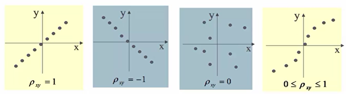
华中科技大学《数字信号分析理论实践》第五单元 信号的时差域分析 学习总结记录 信号相关函数的概念 信号相关分析 (Cross-correlation) 是一种分析两个信号之间或一个信号自身的时间依存关系和相似程度的方法ρ x y ( τ ) = ∫ − ∞ + ∞ x ( t ) y ( t − τ ) d t [ ∫ − ∞ + ∞ x 2 ( t ) d t ∫ − ∞ + ∞ y 2 ( t ) d t ] 1 / 2 \rho_{xy}(\tau)=\frac{\int_{-\infty}^{+\infty}x(t)y(t-\tau)dt}{[{\int_{-\infty}^{+\infty}x^2(t)dt\int_{-\infty}^{+\infty}y^2(t)dt]}^{1/2}} ρxy(τ)=[∫−∞+∞x2(t)dt∫−∞+∞y2(t)dt]1/2∫−∞+∞x(t)y(t−τ)dt 变量相关的概念 统计学中用相关系数来描述变量 x , y x,y x,y 之间的相关性,它是两随机变量之积的数学期望,表征了 x , y x,y x,y 间的关联程度
ρ
x
y
=
c
x
y
σ
x
σ
y
=
E
[
(
x
−
μ
x
)
(
y
−
μ
y
)
]
{
E
[
(
x
−
μ
x
)
2
]
E
[
(
y
−
μ
y
)
2
]
}
1
/
2
\rho_{xy}=\frac{c_{xy}}{\sigma_x\sigma_y}=\frac{E[(x-\mu_x)(y-\mu_y)]}{\{E[(x-\mu_x)^2]E[(y-\mu_y)^2]\}^{1/2}}
ρxy=σxσycxy={E[(x−μx)2]E[(y−μy)2]}1/2E[(x−μx)(y−μy)] 波形相关的概念(相关函数) 如果所研究的变量 x , y x,y x,y 是与时间有关的函数,即 x ( t ) x(t) x(t) 与 y ( t ) y(t) y(t) ,则其相关系数也是随其相对时刻变化的函数这时可以引入一个与相对时间差 τ \tau τ 有关的量,称为函数的相关系数或相关函数,有ρ x y ( τ ) = ∫ − ∞ + ∞ x ( t ) y ( t − τ ) d t [ ∫ − ∞ + ∞ x 2 ( t ) d t ∫ − ∞ + ∞ y 2 ( t ) d t ] 1 / 2 \rho_{xy}(\tau)=\frac{\int_{-\infty}^{+\infty}x(t)y(t-\tau)dt}{[{\int_{-\infty}^{+\infty}x^2(t)dt\int_{-\infty}^{+\infty}y^2(t)dt]}^{1/2}} ρxy(τ)=[∫−∞+∞x2(t)dt∫−∞+∞y2(t)dt]1/2∫−∞+∞x(t)y(t−τ)dt 相关函数反映了两个信号在时移的相关性工程上,人们关心的是信号不同时刻的相似程度,但不太关心其具体值,这时相关函数可简化为R x y ( τ ) = ∫ − ∞ + ∞ x ( t ) y ( t + τ ) d t R_{xy}(\tau)=\int_{-\infty}^{+\infty}x(t)y(t+\tau)dt Rxy(τ)=∫−∞+∞x(t)y(t+τ)dt [FileName,PathName] = uigetfile('*.mp3','Select mp3 File'); abc = fullfile(PathName,FileName); [y,Fs] = audioread(abc); figure subplot(211); plot(y); s = xcorr(y,'unbiased'); subplot(212); plot(s);图形说明,找不到回波音频,随便找了一个 MP3 文件扔进去  N = 1024;
T = 0.2;
t = linspace(0,T,N);
n = randn(1,N);
subplot(211)
plot(t,n);
r = xcorr(n,'unbiased');
t1 = linspace(-T,T,2*N-1);
subplot(212);
plot(t1,r);
N = 1024;
T = 0.2;
t = linspace(0,T,N);
n = randn(1,N);
subplot(211)
plot(t,n);
r = xcorr(n,'unbiased');
t1 = linspace(-T,T,2*N-1);
subplot(212);
plot(t1,r);
 N = 1024;
T = 0.2;
t = linspace(0,T,N);
s1 = sin(2*3.14*50*t);
subplot(311)
plot(t,s1);
s2 = square(2*pi*50*t,60);
subplot(312)
plot(t,s2);
r = xcorr(s1,s2,'unbiased');
t1 = linspace(-T,T,2*N-1);
subplot(313);
plot(t1,r);
ylim([-0.5,0.5])
grid on
两个非同频率的周期信号互不相关,相乘积分等于0
N = 1024;
T = 0.2;
t = linspace(0,T,N);
s1 = sin(2*3.14*50*t);
subplot(311)
plot(t,s1);
s2 = square(2*pi*50*t,60);
subplot(312)
plot(t,s2);
r = xcorr(s1,s2,'unbiased');
t1 = linspace(-T,T,2*N-1);
subplot(313);
plot(t1,r);
ylim([-0.5,0.5])
grid on
两个非同频率的周期信号互不相关,相乘积分等于0  N = 1024;
T = 0.2;
t = linspace(0,T,N);
s1 = sin(2*3.14*50*t);
subplot(311)
plot(t,s1);
s2 = sin(2*3.14*100*t);
subplot(312)
plot(t,s2);
r = xcorr(s1,s2,'unbiased');
t1 = linspace(-T,T,2*N-1);
subplot(313);
plot(t1,r);
ylim([-0.5,0.5])
grid on
N = 1024;
T = 0.2;
t = linspace(0,T,N);
s1 = sin(2*3.14*50*t);
subplot(311)
plot(t,s1);
s2 = sin(2*3.14*100*t);
subplot(312)
plot(t,s2);
r = xcorr(s1,s2,'unbiased');
t1 = linspace(-T,T,2*N-1);
subplot(313);
plot(t1,r);
ylim([-0.5,0.5])
grid on
建议去看原视频,有随着相位改变信号移动的图 相关函数的数学计算方法 相关函数公式R x y ( τ ) = ∫ − ∞ + ∞ x ( t ) y ( t + τ ) d t R_{xy}(\tau)=\int_{-\infty}^{+\infty}x(t)y(t+\tau)dt Rxy(τ)=∫−∞+∞x(t)y(t+τ)dt 数字信号离散计算公式R x y ( k ) = ∑ 0 N − 1 x ( n ) y ( n + k ) k = 0 , 1 , … , N − 1 R_{xy}(k)=\sum_{0}^{N-1}x(n)y(n+k)k=0,1,\dots,N-1 Rxy(k)=0∑N−1x(n)y(n+k)k=0,1,…,N−1 双重循环计算量大 快速算法:频域相乘等于时域卷积 x ( n ) → F F T X ( k ) x(n)\overset{FFT}{\rightarrow}X(k) x(n)→FFTX(k) y ( n ) → F F T Y ( k ) y(n)\overset{FFT}{\rightarrow}Y(k) y(n)→FFTY(k) ⇒ R ( k ) = X ( k ) Y ‾ ( k ) ⇒ R ( k ) → I F F T r ( n ) \Rightarrow R(k)=X(k)\overline{Y}(k)\Rightarrow R(k)\overset{IFFT}{\rightarrow}r(n) ⇒R(k)=X(k)Y(k)⇒R(k)→IFFTr(n) N = 1024; T = 0.2; t = linspace(0,T,N); y = sin(2*3.14*50*t); subplot(311) plot(t,y); s1 = xcorr(y,'unbiased'); % 加上无偏的参数 s2 = xcorr(y); t1 = linspace(-T,T,2*N-1); subplot(312) plot(t1,s1); subplot(313) plot(t1,s2); FFT 计算引入周期延拓问题,为了避免重叠失真,补等宽的零,导致另外一个问题,相关系数越来越小,以零值为中心向两边衰减,因此要加上无偏来修正 相关分析应用——声波传播速度测量,雷达测距,相关滤波
N = 1024;
T = 0.2;
t = linspace(0,T,N);
s = sin(2*3.14*50*t);
subplot(411)
plot(t,s);
n = randn(1,N);
subplot(412)
plot(t,n);
y = s + n;
subplot(413);
plot(t,y);
r = xcorr(y,'unbiased'); % 加上无偏的参数
t1 = linspace(-T,T,2*N-1);
subplot(414);
plot(t1,r);
相关分析应用——声波传播速度测量,雷达测距,相关滤波
N = 1024;
T = 0.2;
t = linspace(0,T,N);
s = sin(2*3.14*50*t);
subplot(411)
plot(t,s);
n = randn(1,N);
subplot(412)
plot(t,n);
y = s + n;
subplot(413);
plot(t,y);
r = xcorr(y,'unbiased'); % 加上无偏的参数
t1 = linspace(-T,T,2*N-1);
subplot(414);
plot(t1,r);

|


【本文地址】
今日新闻 |
推荐新闻 |