【神经网络】(6) 卷积神经网络(VGG16),案例:鸟类图片4分类 |
您所在的位置:网站首页 › vgg16代码 › 【神经网络】(6) 卷积神经网络(VGG16),案例:鸟类图片4分类 |
【神经网络】(6) 卷积神经网络(VGG16),案例:鸟类图片4分类
|
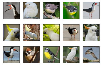
各位同学好,今天和大家分享一下TensorFlow2.0中的VGG16卷积神经网络模型,案例:现在有四种鸟类的图片各200张,构建卷积神经网络,预测图片属于哪个分类。 1. 数据加载将鸟类图片按类分开存放,使用tf.keras.preprocessing.image_dataset_from_directory()函数分批次读取图片数据,统一指定图片加载进来的大小224*224,指定参数label_model,'int'代表目标值y是数值类型,即0, 1, 2, 3等;'categorical'代表onehot类型,对应索引的值为1,如图像属于第二类则表示为0,1,0,0,0;'binary'代表二分类。 import numpy as np import tensorflow as tf from tensorflow import keras from tensorflow.keras import Sequential, optimizers, layers, Model #(1)数据加载 def get_data(height, width, batchsz): # 获取训练集数据 filepath1 = 'C:/Users/admin/.spyder-py3/test/数据集/4种鸟分类/new_data/train' train_ds = tf.keras.preprocessing.image_dataset_from_directory( filepath1, # 指定训练集数据路径 label_mode = 'categorical', # 进行onehot编码 image_size = (height, width), # 对图像risize batch_size = batchsz, # 每次迭代取32个数据 ) # 获取验证集数据 filepath2 = 'C:/Users/admin/.spyder-py3/test/数据集/4种鸟分类/new_data/val' val_ds = tf.keras.preprocessing.image_dataset_from_directory( filepath1, # 指定训练集数据路径 label_mode = 'categorical', image_size = (height, width), # 对图像risize batch_size = batchsz, # 每次迭代取32个数据 ) # 获取测试集数据 filepath2 = 'C:/Users/admin/.spyder-py3/test/数据集/4种鸟分类/new_data/test' test_ds = tf.keras.preprocessing.image_dataset_from_directory( filepath1, # 指定训练集数据路径 label_mode = 'categorical', image_size = (height, width), # 对图像risize batch_size = batchsz, # 每次迭代取32个数据 ) # 返回数据集 return train_ds, val_ds, test_ds # 数据读取函数,返回训练集、验证集、测试集 train_ds, val_ds, test_ds = get_data(height=224, width=224, batchsz=32) # 查看有哪些分类 class_names = train_ds.class_names print('类别有:', class_names) # 类别有: ['Bananaquit', 'Black Skimmer', 'Black Throated Bushtiti', 'Cockatoo'] # 查看数据集信息 sample = next(iter(train_ds)) #每次取出一个batch的训练数据 print('x_batch.shape:', sample[0].shape, 'y_batch.shape:',sample[1].shape) # x_batch.shape: (128, 224, 224, 3) y_batch.shape: (128, 4) print('y[:5]:', sample[1][:5]) # 查看前五个目标值 2. 数据预处理使用.map()函数转换数据集中所有x和y的类型,并将每张图象的像素值映射到[-1,1]之间,打乱训练集数据的顺序.shuffle(),但不改变特征值x和标签值y之间的对应关系。iter()生成迭代器,配合next()每次运行取出训练集中的一个batch数据。 #(2)显示图像 import matplotlib.pyplot as plt for i in range(15): plt.subplot(3,5,i+1) plt.imshow(sample[0][i]/255.0) # sample[0]代表取出的一个batch的所有图像信息,映射到[0,1]之间显示图像 plt.xticks([]) # 不显示xy轴坐标刻度 plt.yticks([]) plt.show() #(3)数据预处理 # 定义预处理函数 def processing(x, y): x = 2 * tf.cast(x, dtype=tf.float32)/255.0 - 1 #映射到[-1,1]之间 y = tf.cast(y, dtype=tf.int32) # 转换数据类型 return x,y # 对所有数据集预处理 train_ds = train_ds.map(processing).shuffle(10000) val_ds = val_ds.map(processing) test_ds = test_ds.map(processing) # 再次查看数据信息 sample = next(iter(train_ds)) #每次取出一个batch的训练数据 print('x_batch.shape:', sample[0].shape, 'y_batch.shape:',sample[1].shape) # x_batch.shape: (128, 224, 224, 3) y_batch.shape: (128, 4) print('y[:5]:', sample[1][:5]) # 查看前五个目标值 # [[0 0 1 0], [1 0 0 0], [0 1 0 0], [0 1 0 0], [1 0 0 0]]鸟类图像如下:
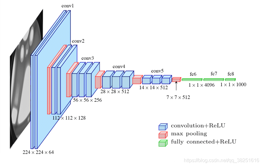
VGG16的模型框架如下图所示,原理见下文:深度学习-VGG16原理详解 。
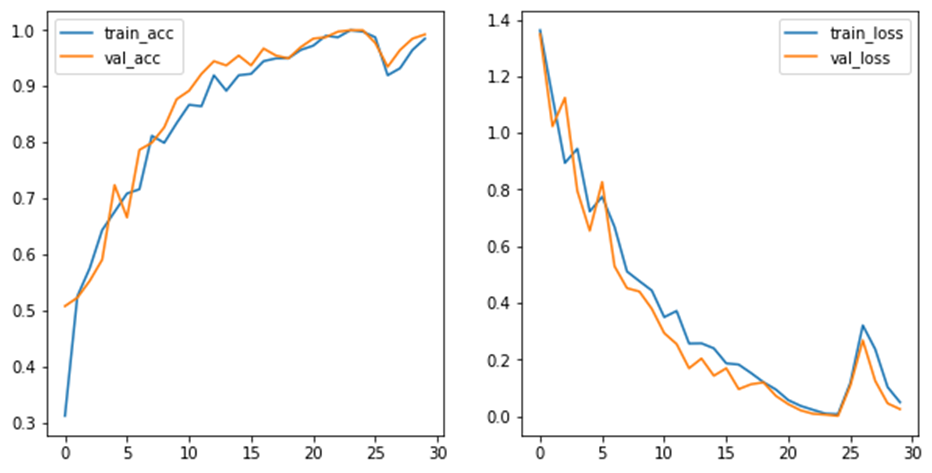
1)输入图像尺寸为224x224x3,经64个通道为3的3x3的卷积核,步长为1,padding=same填充,卷积两次,再经ReLU激活,输出的尺寸大小为224x224x64 2)经max pooling(最大化池化),滤波器为2x2,步长为2,图像尺寸减半,池化后的尺寸变为112x112x64 3)经128个3x3的卷积核,两次卷积,ReLU激活,尺寸变为112x112x128 4)max pooling池化,尺寸变为56x56x128 5)经256个3x3的卷积核,三次卷积,ReLU激活,尺寸变为56x56x256 6)max pooling池化,尺寸变为28x28x256 7)经512个3x3的卷积核,三次卷积,ReLU激活,尺寸变为28x28x512 8)max pooling池化,尺寸变为14x14x512 9)经512个3x3的卷积核,三次卷积,ReLU,尺寸变为14x14x512 10)max pooling池化,尺寸变为7x7x512 11)然后Flatten(),将数据拉平成向量,变成一维51277=25088。 11)再经过两层1x1x4096,一层1x1x1000的全连接层(共三层),经ReLU激活 12)最后通过softmax输出1000个预测结果 下面通过代码来实现,这里我们需要的是4分类,因此把最后的1000个预测结果改为4既可。 #(4)构建CNN-VGG16 def VGG16(input_shape=(224,224,3), output_shape=4): # 输入层 input_tensor = keras.Input(shape=input_shape) # unit1 # 卷积层 x = layers.Conv2D(64, (3,3), activation='relu', strides=1, padding='same')(input_tensor) # [224,224,64] # 卷积层 x = layers.Conv2D(64, (3,3), activation='relu' , strides=1, padding='same')(x) #[224,224,64] # 池化层,size变成1/2 x = layers.MaxPool2D(pool_size=(2,2), strides=(2,2))(x) #[112,112,64] # unit2 # 卷积层 x = layers.Conv2D(128, (3,3), activation='relu', strides=1, padding='same')(x) #[112,112,128] # 卷积层 x = layers.Conv2D(128, (3,3), activation='relu', strides=1, padding='same')(x) #[112,112,128] # 池化层 x = layers.MaxPool2D(pool_size=(2,2), strides=(2,2))(x) #[56,56,128] # unit3 # 卷积层 x = layers.Conv2D(256, (3,3), activation='relu', strides=1, padding='same')(x) #[56,56,256] # 卷积层 x = layers.Conv2D(256, (3,3), activation='relu', strides=1, padding='same')(x) #[56,56,256] # 卷积层 x = layers.Conv2D(256, (3,3), activation='relu', strides=1, padding='same')(x) #[56,56,256] # 池化层 x = layers.MaxPool2D(pool_size=(2,2), strides=(2,2))(x) #[28,28,256] # unit4 # 卷积层 x = layers.Conv2D(512, (3,3), activation='relu', strides=1, padding='same')(x) #[28,28,512] # 卷积层 x = layers.Conv2D(512, (3,3), activation='relu', strides=1, padding='same')(x) #[28,28,512] # 卷积层 x = layers.Conv2D(512, (3,3), activation='relu', strides=1, padding='same')(x) #[28,28,512] # 池化层 x = layers.MaxPool2D(pool_size=(2,2), strides=(2,2))(x) #[14,14,512] # unit5 # 卷积层 x = layers.Conv2D(512, (3,3), activation='relu', strides=1, padding='same')(x) #[14,14,512] # 卷积层 x = layers.Conv2D(512, (3,3), activation='relu', strides=1, padding='same')(x) #[14,14,512] # 卷积层 x = layers.Conv2D(512, (3,3), activation='relu', strides=1, padding='same')(x) #[14,14,512] # 池化层 x = layers.MaxPool2D(pool_size=(2,2), strides=(2,2))(x) #[7,7,512] # uint6 # Flatten层 x = layers.Flatten()(x) #压平[None,4096] # 全连接层 x = layers.Dense(4096, activation='relu')(x) #[None,4096] # 全连接层 x = layers.Dense(4096, activation='relu')(x) #[None,4096] # 输出层,输出结果不做softmax output_tensor = layers.Dense(output_shape)(x) #[None,4] # 构建模型 model = Model(inputs=input_tensor, outputs=output_tensor) # 返回模型 return model # 构建VGG16模型 model = VGG16() # 查看模型结构 model.summary()该网络构架如下 Model: "model" _________________________________________________________________ Layer (type) Output Shape Param # ================================================================= input_1 (InputLayer) [(None, 224, 224, 3)] 0 conv2d (Conv2D) (None, 224, 224, 64) 1792 conv2d_1 (Conv2D) (None, 224, 224, 64) 36928 max_pooling2d (MaxPooling2D (None, 112, 112, 64) 0 ) conv2d_2 (Conv2D) (None, 112, 112, 128) 73856 conv2d_3 (Conv2D) (None, 112, 112, 128) 147584 max_pooling2d_1 (MaxPooling (None, 56, 56, 128) 0 2D) conv2d_4 (Conv2D) (None, 56, 56, 256) 295168 conv2d_5 (Conv2D) (None, 56, 56, 256) 590080 conv2d_6 (Conv2D) (None, 56, 56, 256) 590080 max_pooling2d_2 (MaxPooling (None, 28, 28, 256) 0 2D) conv2d_7 (Conv2D) (None, 28, 28, 512) 1180160 conv2d_8 (Conv2D) (None, 28, 28, 512) 2359808 conv2d_9 (Conv2D) (None, 28, 28, 512) 2359808 max_pooling2d_3 (MaxPooling (None, 14, 14, 512) 0 2D) conv2d_10 (Conv2D) (None, 14, 14, 512) 2359808 conv2d_11 (Conv2D) (None, 14, 14, 512) 2359808 conv2d_12 (Conv2D) (None, 14, 14, 512) 2359808 max_pooling2d_4 (MaxPooling (None, 7, 7, 512) 0 2D) flatten (Flatten) (None, 25088) 0 dense (Dense) (None, 4096) 102764544 dense_1 (Dense) (None, 4096) 16781312 dense_2 (Dense) (None, 4) 16388 ================================================================= Total params: 134,276,932 Trainable params: 134,276,932 Non-trainable params: 0 _________________________________________________________________ 4. 网络编译在网络编译时.compile(),指定损失loss采用交叉熵损失,设置参数from_logits=True,由于网络的输出层没有使用softmax函数将输出的实数转为概率,参数设置为True时,会自动将logits的实数转为概率值,再和真实值计算损失,这里的真实值y是经过onehot编码之后的结果。 #(5)模型配置 # 设置优化器 opt = optimizers.Adam(learning_rate=1e-4) # 学习率 model.compile(optimizer=opt, #学习率 loss=keras.losses.CategoricalCrossentropy(from_logits=True), #损失 metrics=['accuracy']) #评价指标 # 训练,给定训练集、验证集 history = model.fit(train_ds, validation_data=val_ds, epochs=30) #迭代30次 #(6)循环结束后绘制损失和准确率的曲线 # ==1== 准确率 train_acc = history.history['accuracy'] #训练集准确率 val_acc = history.history['val_accuracy'] #验证集准确率 # ==2== 损失 train_loss = history.history['loss'] #训练集损失 val_loss = history.history['val_loss'] #验证集损失 # ==3== 绘图 epochs_range = range(len(train_acc)) plt.figure(figsize=(10,5)) # 准确率 plt.subplot(1,2,1) plt.plot(epochs_range, train_acc, label='train_acc') plt.plot(epochs_range, val_acc, label='val_acc') plt.legend() # 损失曲线 plt.subplot(1,2,2) plt.plot(epochs_range, train_loss, label='train_loss') plt.plot(epochs_range, val_loss, label='val_loss') plt.legend() 5. 结果展示如图可见网络效果预测较好,在迭代至25次左右时网络准确率达到99%左右,如果迭代次数较多的话,可考虑在编译时使用early stopping保存最优权重,若后续网络效果都没有提升就可以提早停止网络,节约训练时间。
训练过程中的损失和准确率如下 Epoch 1/30 13/13 [==============================] - 7s 293ms/step - loss: 1.3627 - accuracy: 0.3116 - val_loss: 1.3483 - val_accuracy: 0.5075 Epoch 2/30 13/13 [==============================] - 3s 173ms/step - loss: 1.1267 - accuracy: 0.5251 - val_loss: 1.0235 - val_accuracy: 0.5226 ------------------------------------------------------------------------------------------ 省略N行 ------------------------------------------------------------------------------------------ Epoch 26/30 13/13 [==============================] - 2s 174ms/step - loss: 0.1184 - accuracy: 0.9874 - val_loss: 0.1093 - val_accuracy: 0.9774 Epoch 27/30 13/13 [==============================] - 2s 174ms/step - loss: 0.3208 - accuracy: 0.9196 - val_loss: 0.2678 - val_accuracy: 0.9347 Epoch 28/30 13/13 [==============================] - 2s 172ms/step - loss: 0.2366 - accuracy: 0.9322 - val_loss: 0.1247 - val_accuracy: 0.9648 Epoch 29/30 13/13 [==============================] - 3s 173ms/step - loss: 0.1027 - accuracy: 0.9648 - val_loss: 0.0453 - val_accuracy: 0.9849 Epoch 30/30 13/13 [==============================] - 3s 171ms/step - loss: 0.0491 - accuracy: 0.9849 - val_loss: 0.0250 - val_accuracy: 0.9925 6. 其他方法如果想更灵活的计算损失和准确率,可以不使用.compile(),.fit()函数。在模型构建完之后,自己敲一下代码实现前向传播,同样能实现模型训练效果。下面的代码可以代替第4小节中的第(5)步 # 指定优化器 optimizer = optimizers.Adam(learning_rate=1e-5) # 记录训练和测试过程中的每个batch的准确率和损失 train_acc = [] train_loss = [] val_acc = [] val_loss = [] # 大循环 for epochs in range(30): #循环30次 train_total_sum=0 train_total_loss=0 train_total_correct=0 val_total_sum=0 val_total_loss=0 val_total_correct=0 #(5)网络训练 for step, (x,y) in enumerate(train_ds): #每次从训练集中取出一个batch # 梯度跟踪 with tf.GradientTape() as tape: # 前向传播 logits = model(x) # 输出属于每个分类的实数值 # 计算准确率 prob = tf.nn.softmax(logits, axis=1) # 计算概率 predict = tf.argmax(prob, axis=1, output_type=tf.int32) # 概率最大值的下标 correct = tf.cast(tf.equal(predict, y), dtype=tf.int32) # 对比预测值和真实值,将结果从布尔类型转变为1和0 correct = tf.reduce_sum(correct) # 计算一共预测对了几个 total = x.shape[0] # 每次迭代有多少参与进来 train_total_sum += total #记录一共有多少个样本参与了循环 train_total_correct += correct #记录一整次循环下来预测对了几个 acc = correct/total # 每一个batch的准确率 train_acc.append(acc) # 将每一个batch的准确率保存下来 # 计算损失 y = tf.one_hot(y, depth=4) # 对真实值进行onehot编码,分为4类 loss = tf.losses.categorical_crossentropy(y, logits, from_logits=True) # 将预测值放入softmax种再计算损失 # 求每个batch的损失均值 loss_avg = tf.reduce_mean(loss, axis=1) # 记录总损失 train_total_loss += tf.reduce_sum(loss) #记录每个batch的损失 # 梯度计算,因变量为loss损失,自变量为模型中所有的权重和偏置 grads = tape.gradient(loss_avg, model.trainable_variables) # 梯度更新,对所有的权重和偏置更新梯度 optimizer.apply_gradients(zip(grads, model.trainable_variables)) # 每20个batch打印一次损失和准确率 if step%20 == 0: print('train', 'step:', step, 'loss:', loss_avg, 'acc:', acc) # 记录每次循环的损失和准确率 train_acc.append(train_total_correct/train_total_sum) # 总预测对的个数除以总个数,平均准确率 train_loss.append(train_total_loss/train_total_sum) # 总损失处于总个数,得平均损失 #(6)网络测试 for step, (x, y) in enumerate(val_ds): #每次取出一个batch的验证数据 # 前向传播 logits = model(x) # 计算准确率 prob = tf.nn.softmax(logits, axis=1) # 计算概率 predict = tf.argmax(prob, axis=1, output_type=tf.int32) # 概率最大值的下标 correct = tf.cast(tf.equal(predict, y), dtype=tf.int32) # 对比预测值和真实值,将结果从布尔类型转变为1和0 correct = tf.reduce_sum(correct) # 计算一共预测对了几个 val_total_correct += correct # 计算整个循环预测对了几个 total = x.shape[0] # 每次迭代有多少参与进来 val_total_sum += total # 整个循环有多少参与进来 acc = correct/total # 每一个batch的准确率 val_acc.append(acc) # 将每一个batch的准确率保存下来 # 计算损失 y = tf.one_hot(y, depth=4) # 对真实值进行onehot编码,分为4类 loss = tf.losses.categorical_crossentropy(y, logits, from_logits=True) # 将预测值放入softmax种再计算损失 # 求每个batch的损失均值 loss_avg = tf.reduce_mean(loss, axis=1) # 记录总损失 val_total_loss += tf.reduce_sum(loss) # 每10个btch打印一次准确率和损失 if step%10 == 0: print('val', 'step:', step, 'loss:', loss_avg, 'acc:', acc) # 记录每次循环的损失和准确率 val_acc.append(val_total_correct/val_total_sum) # 总预测对的个数除以总个数,平均准确率 val_loss.append(val_total_loss/val_total_sum) # 总损失处于总个数,得平均损失 |
【本文地址】
今日新闻 |
推荐新闻 |