TensorFlow2利用Fashion |
您所在的位置:网站首页 › tensorflow2图像分类训练 › TensorFlow2利用Fashion |
TensorFlow2利用Fashion
|
1. 导入所需的库
import tensorflow as tf
import numpy as np
import matplotlib.pyplot as plt
for i in [tf, np]:
print(i.__name__,": ",i.__version__,sep="")
输出: tensorflow: 2.2.0 numpy: 1.17.4 2. 导入Fashion_MNIST数据集 fashion_mnist = tf.keras.datasets.fashion_mnist (trainImages, trainLabels),(testImages, testLabels) = fashion_mnist.load_data() for i in [trainImages, trainLabels, testImages, testLabels]: print(i.shape)输出: (60000, 28, 28) (60000,) (10000, 28, 28) (10000,)从上面输出可以看出,Fashion MNIST数据集训练集共有6万张图像,测试集有1万张图像,并且每张图像大小为28*28。(从后面的分析也可以发现图像是三通道的,即彩色的) 导入的数据是NumPy array结构,数据中像素值是0至255之间的值,标签值是从0至9之间的数,并且分别对应如下衣物名称: 标签值类别0T-shirt/top1Trouser2Pullover3Dress4Coat5Sandal6Shirt7Sneaker8Bag9Ankle boot classNames = ['T-shirt/top', 'Trouser', 'Pullover', 'Dress', 'Coat','Sandal', 'Shirt', 'Sneaker', 'Bag', 'Ankle boot'] 3. 数据初探查看某一样本数据所代表的图像,例如下面例子查看第11张图像,结果显示一件T恤 plt.figure() plt.imshow(trainImages[10]) plt.colorbar() plt.grid(False) plt.show()
查看fashion_mnist数据集中的样本发现,每个样本的像素值是0至255之间的值,因此在训练网络之前需要做归一化的操作。 trainImages = trainImages/255.0 testImages = testImages/255.0查看前25个数据所代表的图像 plt.figure(figsize=(12,12)) for i in range(25): plt.subplot(5,5,i+1) plt.xticks([]) plt.yticks([]) plt.imshow(trainImages[i], cmap=plt.cm.binary) plt.xlabel(classNames[trainLabels[i]]) plt.show()输出:
构建模型分为:模型结构构建和模型编译两步 4.1 模型结构构建 model = tf.keras.Sequential([ tf.keras.layers.Flatten(input_shape=(28,28)), tf.keras.layers.Dense(128, activation="relu"), tf.keras.layers.Dense(10) ]) model.summary()输出: Model: "sequential" _________________________________________________________________ Layer (type) Output Shape Param # ================================================================= flatten (Flatten) (None, 784) 0 _________________________________________________________________ dense (Dense) (None, 128) 100480 _________________________________________________________________ dense_1 (Dense) (None, 10) 1290 ================================================================= Total params: 101,770 Trainable params: 101,770 Non-trainable params: 0 _________________________________________________________________模型中第一层tf.keras.layers.Flatten将输入图像从二维的28*28拉平成一维的784向量。后面加入了两层的全连接层(FC)。 4.2 模型编译编译模型过程即是加入一些参数或进行一些设置,例如指定优化器、损失函数,以及模型评估参数等 model.compile(optimizer="adam", loss=tf.keras.losses.SparseCategoricalCrossentropy(from_logits=True), metrics=["accuracy"]) 5. 训练模型训练模型时需要指定训练数据(包括数据特征和数据标签),指定训练轮数 5.1 模型训练 model.fit(trainImages,trainLabels,epochs=10) Epoch 1/10 1875/1875 [==============================] - 2s 905us/step - loss: 0.4954 - accuracy: 0.8273 Epoch 2/10 1875/1875 [==============================] - 2s 897us/step - loss: 0.3776 - accuracy: 0.8648 Epoch 3/10 1875/1875 [==============================] - 1s 749us/step - loss: 0.3385 - accuracy: 0.8776 Epoch 4/10 1875/1875 [==============================] - 1s 771us/step - loss: 0.3140 - accuracy: 0.8842 Epoch 5/10 1875/1875 [==============================] - 1s 766us/step - loss: 0.2961 - accuracy: 0.8909 Epoch 6/10 1875/1875 [==============================] - 1s 793us/step - loss: 0.2839 - accuracy: 0.8941 Epoch 7/10 1875/1875 [==============================] - 1s 767us/step - loss: 0.2697 - accuracy: 0.8991 Epoch 8/10 1875/1875 [==============================] - 1s 780us/step - loss: 0.2586 - accuracy: 0.9034 Epoch 9/10 1875/1875 [==============================] - 1s 760us/step - loss: 0.2482 - accuracy: 0.9082 Epoch 10/10 1875/1875 [==============================] - 1s 789us/step - loss: 0.2415 - accuracy: 0.9090 Out[54]:如上模型训练10轮后可以看出,训练集上糖度达到了90.98% 5.2 模型评估模型训练完成后需要在测试集上进行测试,求得精度 testLoss, testAcc = model.evaluate(testImages, testLabels, verbose=2) print(testAcc)输出: 313/313 - 0s - loss: 0.3476 - accuracy: 0.8803 0.880299985408783对比模型在训练集和测试集上的糖度发现,测试集上的糖度稍低于训练集,这是神经网络最常见的问题之一,即过拟合。如何防止过拟合,请参考后面的文章。 5.3 利用训练好的模型进行预测 probabilityModel = tf.keras.Sequential([model, tf.keras.layers.Softmax()]) predictions = probabilityModel.predict(testImages) print(predictions[0]) print(np.argmax(predictions[0]))输出: [5.1641495e-05 2.5693788e-07 3.9040547e-08 2.5029462e-07 2.5109449e-08 7.9626171e-04 4.5378929e-06 1.5559687e-02 9.3849840e-06 9.8357797e-01] 9 plt.figure() plt.imshow(trainImages[0]) plt.colorbar() plt.grid(False) plt.show() print(classNames[testLabels[0]])输出:
可以发现预测结果与真实图像是一致的。 5.4 可视化预测结果 def plot_image(i, predictions_array, true_label, img): predictions_array, true_label, img = predictions_array, true_label[i], img[i] plt.grid(False) plt.xticks([]) plt.yticks([]) plt.imshow(img, cmap=plt.cm.binary) predicted_label = np.argmax(predictions_array) if predicted_label == true_label: color = 'blue' else: color = 'red' plt.xlabel("{} {:2.0f}% ({})".format(classNames[predicted_label], 100*np.max(predictions_array), classNames[true_label]), color=color) def plot_value_array(i, predictions_array, true_label): predictions_array, true_label = predictions_array, true_label[i] plt.grid(False) plt.xticks(range(10)) plt.yticks([]) thisplot = plt.bar(range(10), predictions_array, color="#777777") plt.ylim([0, 1]) predicted_label = np.argmax(predictions_array) thisplot[predicted_label].set_color('red') thisplot[true_label].set_color('blue')单独查看某一张预测结果: i = 1000 plt.figure(figsize=(6,3)) plt.subplot(1,2,1) plot_image(i, predictions[i], testLabels, testImages) plt.subplot(1,2,2) plot_value_array(i, predictions[i], testLabels) plt.show()输出:
输出:
批量查看前15张的预测结果: num_rows = 5 num_cols = 3 num_images = num_rows*num_cols plt.figure(figsize=(2*2*num_cols, 2*num_rows)) for i in range(num_images): plt.subplot(num_rows, 2*num_cols, 2*i+1) plot_image(i, predictions[i], testLabels, testImages) plt.subplot(num_rows, 2*num_cols, 2*i+2) plot_value_array(i, predictions[i], testLabels) plt.tight_layout() plt.show()输出:
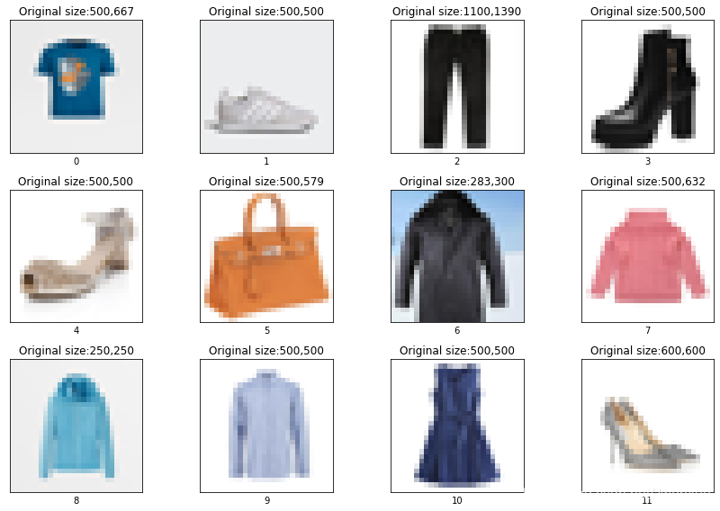
从上面结果可以看出,第13张被预测错了。很明显应该是运动鞋(Sneaker),而被预测成了凉鞋(Sandal)。 6. 使用模型预测自己的图片 6.1 获取检测样本从网上找12张图片,用训练的模型进行预测,观察预测效果如何? from PIL import Image, ImageOps import matplotlib.pyplot as plt import numpy as np plt.figure(figsize=(12, 8)) for i in range(12): img = Image.open(str(i+1)+".jpg") #img = img.convert("L") #img = np.array(img) shape = img.size img = img.resize((28,28)) plt.subplot(3, 4, i+1) plt.grid(False) plt.xticks([]) plt.yticks([]) plt.imshow(img, cmap=plt.cm.binary) plt.title("Original size:{},{}".format(str(shape[0]),str(shape[1]))) plt.xlabel(i) plt.tight_layout()输出:
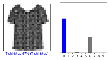
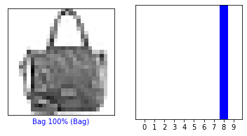
上图所示是从网上随便下载的12张图片,图片上方Original size表示图片的原始大小,为了方便展示统一缩放到28*28。 6.2 检测12张图片并可视化结果 def loadImage(i): from PIL import Image, ImageOps img = Image.open(str(i)+".jpg") img = img.convert("L") # 将彩色图像转换成黑白图像 img = ImageOps.invert(img) # 将图像黑色和白色反转,即为了与Fashion MNIST数据集保持一致,将背景部分转换成白色 img = img.resize((28,28)) # 改变大小为28*28 img = np.array(img) # 转换成NumPy数据形式 img = img/255.0 return img def plot_image(i, img, prediction): plt.grid(False) plt.xticks([]) plt.yticks([]) plt.imshow(img, cmap=plt.cm.binary) predicted_label = np.argmax(prediction) plt.title(i+1) plt.xlabel("Predict:{} {:2.0f}% ".format(classNames[predicted_label], 100*np.max(prediction))) def plot_value_array(i,img, prediction): plt.grid(False) plt.xticks(range(10)) plt.yticks([]) thisplot = plt.bar(range(10), prediction[0], color="#777777") plt.ylim([0, 1]) #predicted_label = np.argmax(probabilityModel.predict(img)[0]) num_rows = 4 num_cols = 3 num_images = num_rows*num_cols plt.figure(figsize=(2*2*num_cols, 2*num_rows)) for i in range(num_images): img = loadImage(i+1) prediction = probabilityModel.predict(np.expand_dims(img,0)) plt.subplot(num_rows, 2*num_cols, 2*i+1) # 绘制原始图像 plot_image(i,img, prediction) plt.subplot(num_rows, 2*num_cols, 2*i+2) # 绘制预测概率分布图 plot_value_array(i,img, prediction) plt.tight_layout() plt.show()输出:
从上图可以看出,第1、2、9、12张都被错误地预测成了包(bag)。第2和12张图像很明显是鞋子,而被错误地预测成了包;此时我们观察Fashion MNIST数据集发现,该数据集中的鞋子的鞋头都超向左边,而本例中第2和12张鞋头都是超右的,最终导致被预测错了。这说明我们的训练的模型“没见过”鞋头超右的样本,而只见过鞋头超左的样本。解决这个问题可以有两种办法: 1. 对训练的数据集做数据增强,例如左右翻转。2. 对第2张和第12张图像翻转后再进行预测显然第1种方法是更科学的方法,此处为了方便我们采用第2种方法再次进行预测。 6.3 翻转图像再次预测 def loadImage(i): from PIL import Image, ImageOps img = Image.open(str(i)+".jpg") img = img.transpose(Image.FLIP_LEFT_RIGHT) # 对图像进行水平翻转 img = img.convert("L") # 将彩色图像转换成黑白图像 img = ImageOps.invert(img) # 将图像黑色和白色反转,即为了与Fashion MNIST数据集保持一致,将背景部分转换成白色 img = img.resize((28,28)) # 改变大小为28*28 img = np.array(img) # 转换成NumPy数据形式 img = img/255.0 return img num_rows = 4 num_cols = 3 num_images = num_rows*num_cols plt.figure(figsize=(2*2*num_cols, 2*num_rows)) for i in range(num_images): img = loadImage(i+1) prediction = probabilityModel.predict(np.expand_dims(img,0)) plt.subplot(num_rows, 2*num_cols, 2*i+1) # 绘制原始图像 plot_image(i,img, prediction) plt.subplot(num_rows, 2*num_cols, 2*i+2) # 绘制预测概率分布图 plot_value_array(i,img, prediction) plt.tight_layout() plt.show()输出:
对于上述结果,我们先仅关注鞋子。第12张水平翻转后分类正确;而第4、5张又被预测错了,第2张还是预测错误,说明图像的方向对结果还是有一定的影响。¶ 写在最后,最好的办法还是训练之前对数据进行数据增强的操作。
|


【本文地址】
今日新闻 |
推荐新闻 |