Visualizations are a great way to show the story that data wants to tell. However, not all visualizations are built the same. My rule of thumb is stick to simple, easy to understand, and well labeled graphs. Line graphs, bar charts, and histograms always work best. The most recognized libraries for visualizations are matplotlib and seaborn. Seaborn is built on top of matplotlib, so it is worth looking at matplotlib first, but in this article we’ll look at matplotlib only. Let’s get started. First, we will import all the libraries we will be working with.

可视化是显示数据要讲述的故事的好方法。 但是，并非所有可视化文件的构建都是相同的。 我的经验法则是坚持简单，易于理解且标签清晰的图形。 折线图，条形图和直方图总是最有效。 最受认可的可视化库是matplotlib和seaborn。 Seaborn是建立在matplotlib之上的，因此值得首先看一下matplotlib，但是在本文中，我们将只看一下matplotlib。 让我们开始吧。 首先，我们将导入将要使用的所有库。

We imported numpy, so we can generate random data. From matplotlib, we imported pyplot. If you are working on visualizations in jupyter notebook, you can call the %matplotlib inline command. This will allow jupyter notebook to display your visualizations directly under the code that was ran. If you’d like an interactive chart, you can call the %matplotlib command. This will allow you to manipulate your visualizations such as zoom in, zoom out, and move them around their axis.

我们导入了numpy，因此我们可以生成随机数据。 从matplotlib中，我们导入了pyplot。 如果要在jupyter Notebook中进行可视化，则可以调用％matplotlib内联命令。 这将使jupyter Notebook在运行的代码下直接显示可视化效果。 如果需要交互式图表，可以调用％matplotlib命令。 这将允许您操纵可视化效果，例如放大，缩小并围绕其轴移动它们。

Fist, lets take a look at histograms on matplotlib. We will look at a normal distribution. Let’s build it with numpy and visualize it with matplotlib.

拳头，让我们看看matplotlib上的直方图。 我们将看一个正态分布。 让我们使用numpy构建它，并使用matplotlib对其进行可视化。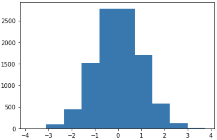

Great! We had a histogram. But, what did we just do? First, we took 10,000 random sample from a distribution of mean 0 and standard deviation of 1. Then, we called the method hist() from matplotlib. Last, we called the show() method to display our figure. However, our histogram looks kind of…squared. Fear not! You can modify the width of each bin with the bins argument. Matplotlib defaults to 10 if an argument isn’t given. There are multiple ways to calculate bins, but I prefer to set it to ‘auto’.

大！ 我们有一个直方图。 但是，我们只是做什么？ 首先，我们从均值为0且标准差为1的分布中抽取了10,000个随机样本。然后，从matplotlib中调用了hist()方法。 最后，我们调用了show()方法来显示我们的图形。 但是，我们的直方图看起来有点...平方。 不要怕！ 您可以使用bins参数修改每个垃圾箱的宽度。 如果未提供参数，则Matplotlib默认为10。 有多种计算垃圾箱的方法，但我更喜欢将其设置为“自动”。

!

！