|
ResNet结构

ResNet的网络结构有:ResNet18、ResNet34、ResNet50、ResNet101、ResNet152.其中ResNet18和ResNet34属于浅层网络,ResNet50、ResNet101、ResNet152属于深层网络。
ResNet创新点
1.超深的网络结构(突破1000层)
2.提出Residual模块
3.使用Batch Normalization加速训练
残差结构
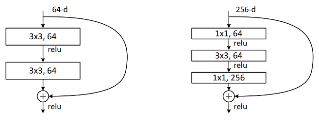
ResNet有两种残差结构,左边这种称为BasicBlock,包含2个3*3的卷积层,用于ResNet18、ResNet34中,右边这种称为Bottleneck,包含3个卷积层,依次为1*1、3*3、1*1,用于ResNet50、ResNet101、ResNet152。
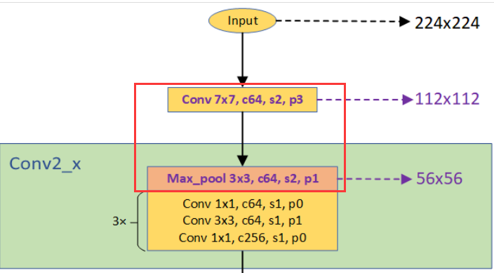
我们把残差结构称为block,每个stage都是由若干个block组成。再由若干stage组成整个网络。这里把开始时7*7的卷积层和3*3的maxpool层称为stem层,除去stem层每种ResNet都是4个stage。图中一个方括号就是一个Block,由若干个Block组成一个stage,图中conv2_x对应stage1,conv3_x对应stage2,conv4_x对应stage3,conv5_x对应stage4.
各ResNet网络都具有以下的共同点:
网络一共有5个卷积组,每个卷积组都进行若干次基本的卷积操作(Conv->BN->ReLU)每个卷积组都会进行一次下采样操作,使特征图的尺寸减半。在卷积组2中使用最大池化进行下采样;在其余4个卷积组中使用卷积进行下采样。每个网络的第一个卷积组都是相同的,卷积核7*7,步长为2。第2-5卷积组均由若干残差结构组成,称为stage1-4.
下面以ResNet34和ResNet50为例介绍网络的结构。
ResNet 34

stem layer

处理流程是:卷积->BN->ReLU->池化->BN->ReLU
卷积:输入图片的尺寸为3*224*224(channel*height*width),使用64个3*7*7的卷积核进行卷积,padding=3,stride=2.输出为64*112*112。
池化:使用64个3*3,padding=1,stride=2的池化单元进行maxpooling,输出为64*56*56。
stage 1
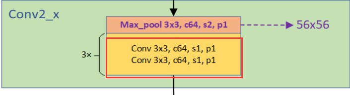
处理流程是:(卷积->BN->ReLU)*3
stage 1由3个BasicBlock组成,每个BasicBlock由两层卷积层组成,每层64个64*3*3的卷积核,stride=1,padding=1。输出仍为64*56*56.
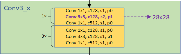
stage 2
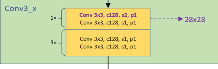
处理流程是:(卷积->BN->ReLU)*4
stage 2由4个BasicBlock组成,与stage 1不同,第一个BasicBlock的卷积层1是128个64*3*3的卷积核,stride=2,padding=1;卷积层2是128个128*3*3的卷积核,stride=1,padding=1.输出128*28*28.
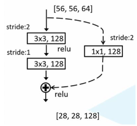
到第一个Block末尾处,需要在output加上residual,但输入为64*56*56,所以在输入和输出之间加一个1*1的卷积层,stride=2,使得输入和输出尺寸一致。(代码中downsample部分)
第二、三、四个BasicBlock由两层卷积层组成,每层128个128*3*3的卷积核,stride=1,padding=1。输出为128*28*28. 由于这些Block没有降低尺寸,residual和输出尺寸相同,所以没有downsample部分。
stage 3-4

stage 3-4与stage 2类似,都使通道数变多,输出尺寸变小。stage 3的输出为256*14*14,stage 4的输出为512*7*7.
了解网络的结构后,我们发现:ResNet中的下采样操作发生在每个Stage的第一个Block或最大池化层,实现方式是操作都是通过在卷积或者池化中取步长为2。
ResNet 50

stem layer
所有ResNet的stem layer均是相同的。
处理流程是:卷积->BN->ReLU->池化->BN->ReLU
卷积:输入图片的尺寸为3*224*224(channel*height*width),使用64个3*7*7的卷积核进行卷积,padding=3,stride=2.输出为64*112*112。
池化:使用3*3,padding=1,stride=2的池化单元进行maxpooling,输出为64*56*56。
stage 1

与Basicblock不同的是,每一个Bottleneck都会在输入和输出之间加上一个卷积层,加入卷积层的原因是使得输入和输出尺寸一致。只不过在stage 1中还没有downsample,这点和Basicblock是相同的。
处理流程是:(卷积->BN->ReLU)*3
stage 1由3个Bottleneck组成,每个Bottleneck由三层卷积层组成,第一层64个1*1的卷积核,stride=1,padding=0。输出为64*56*56;第二层64个64*3*3的卷积核,stride=1,padding=1,输出为64*56*56;第三层256个64*1*1的卷积核,stride=1,padding=0,输出为256*56*56.此操作重复3遍,输出为256*56*56.
stage 2
由4个Bottleneck组成,不同的是第一个Bottleneck,第一层128个1*1的卷积核,stride=1,padding=0,输出为128*56*56;第二层128个128*3*3的卷积核,stride=2,padding=1,输出为128*28*28;第三层512个128*1*1的卷积核,stride=1,padding=0,输出为512*28*28.在第一个Bottleneck输出尺寸发生变化,需要downsample,使用512个1*1,stride=2的卷积层实现。

之后的3个Bottleneck,第一层128个1*1的卷积核,stride=1,padding=1,输出为128*28*28;第二层128个3*3的卷积核,stride=1,padding=1,输出为128*28*28;第三层512个1*1的卷积核,stride=1,padding=0,输出为512*28*28. stride均为1,均不改变图像的尺寸,不需要downsample。
stage 3-4
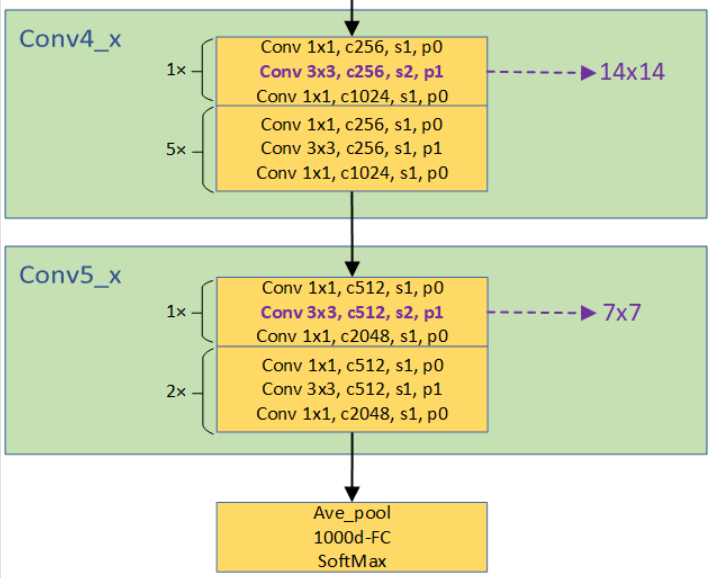
stage 3-4与stage 2类似,都使通道数变多,输出尺寸变小。stage 3的输出为1024*14*14,stage 4的输出为2048*7*7.
我们可以发现:ResNet18/34下采样发生在每个stage(不包括stage 1)的第一个Block的第一个卷积层。ResNet50/101/152下采样发生在每个stage(不包括stage 1)的第一个Block的第二个卷积层。
Batch Normalization(BN)
Batch Normalization的目的
Batch Normalization 的目的是使我们的一批(1个Batch)的特征图满足均值为0,方差为1的高斯分布(正态分布)。通过该方法能够加速网络的收敛并提升准确率。
Batch Normalization的原理
在图像预处理过程中对图像标准化处理,这样可以加速网络的收敛。Batch Normalization的目的就是使我们的feature map满足均值为0,方差为1的分布规律(batch越大越接近整个数据集的分布,效果越好)。计算方法如下:
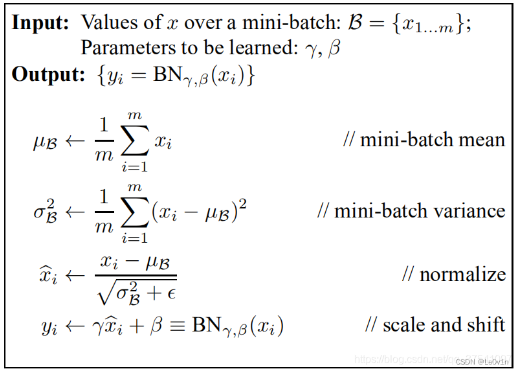
首先计算每个batch同一个通道所有的对应的均值 和方差 和方差 。然后对原参数进行标准化,即可得到经标准化处理后的数值 。然后对原参数进行标准化,即可得到经标准化处理后的数值 ,其中 ,其中  为极小数(防止分母为0)。最后通过 为极小数(防止分母为0)。最后通过  和 和  对特征图的数值进一步调整,其中 和 分别用于调整方差和均值的大小。如果不进行 和 调整,那么整批(Batch)的数据符合均值为0,方差为1的高斯分布规律。 对特征图的数值进一步调整,其中 和 分别用于调整方差和均值的大小。如果不进行 和 调整,那么整批(Batch)的数据符合均值为0,方差为1的高斯分布规律。
均值为0, 方差为1的高斯分布不好吗,为什么还要进行调整? 对于不同的数据集来说,高斯分布不一定是最好的,所以BN有两个可以学习的参数, , 通过反向传播进行学习和更新。 Note:
是用来调整数值分布的方差大小,是用来调节数值均值的位置(均值的中心位置)。这两个参数是在反向传播过程中学习并更新的,而不像均值和方差那样正向传播中更新的。均值和方差的默认值分别为0和1.
我们在预测过程中通常都是输入一张图片进行预测,此时batch size为1,如果再通过上述方法计算均值和方差就没有意义了。所以我们在训练过程中要去不断的计算每个batch的均值和方差,并使用移动平均(moving average)的方法记录统计的均值和方差,在训练完后我们可以近似认为所统计的均值和方差就等于整个训练集的均值和方差。最后在我们验证以及预测过程中,就使用统计得到的均值和方差进行标准化处理。
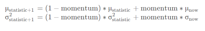
在训练过程中,均值和方差是通过计算当前Batch数据得到的记为 和 和 ,而验证以及预测过程中所使用的均值方差是一个统计量记为 ,而验证以及预测过程中所使用的均值方差是一个统计量记为 和 和 。二者的具体更新策略如下,其中momentum默认为0.1: 。二者的具体更新策略如下,其中momentum默认为0.1:
代码
model
import torch.nn as nn
import torch
class BasicBlock(nn.Module):
# for ResNet-18/34
expansion = 1
def __init__(self, in_channel, out_channel, stride=1, downsample=None, **kwargs):
super(BasicBlock, self).__init__()
# Conv(without bias)->BN->ReLU
self.conv1 = nn.Conv2d(in_channel, out_channel, kernel_size=3, stride=stride, padding=1, bias=False)
self.bn1 = nn.BatchNorm2d(out_channel)
self.relu = nn.ReLU()
self.conv2 = nn.Conv2d(out_channel, out_channel, kernel_size=3, stride=1, padding=1, bias=False)
self.bn2 = nn.BatchNorm2d(out_channel)
self.downsample = downsample
def forward(self, x):
identity = x
if self.downsample is not None:
identity = self.downsample(x)
out = self.conv1(x)
out = self.bn1(out)
out = self.relu(out)
out = self.conv2(out)
out = self.bn2(out)
out += identity
out = self.relu(out)
return out
class Bottleneck(nn.Module):
expansion = 4
def __init__(self, in_channel, out_channel, stride=1, downsample=None, groups=1, width_pre_group=64):
super(Bottleneck, self).__init__()
width = int(out_channel * (width_pre_group/64.)) * groups
self.conv1 = nn.Conv2d(in_channel, width, kernel_size=1, stride=1, bias=False)
self.bn1 = nn.BatchNorm2d(width)
self.conv2 = nn.Conv2d(width, width, groups=groups, kernel_size=3, stride=stride, bias=False, padding=1)
self.bn2 = nn.BatchNorm2d(width)
self.conv3 = nn.Conv2d(width, out_channel*self.expansion, kernel_size=1, stride=1, bias=False)
self.bn3 = nn.BatchNorm2d(out_channel*self.expansion)
self.relu = nn.ReLU(inplace=True)
self.downsample = downsample
def forward(self, x):
identity = x
if self.downsample is not None:
identity = self.downsample(x)
out = self.conv1(x)
out = self.bn1(out)
out = self.relu(out)
out = self.conv2(out)
out = self.bn2(out)
out = self.relu(out)
out = self.conv3(out)
out = self.bn3(out)
out += identity
out = self.relu(out)
return out
class ResNet(nn.Module):
def __init__(self, block, blocks_num, num_classes=1000, include_top=True, groups=1, width_per_group=64):
super(ResNet, self).__init__()
self.include_top = include_top
self.in_channel = 64
self.groups = groups
self.width_per_group = width_per_group
self.conv1 = nn.Conv2d(3, self.in_channel, kernel_size=7, stride=2, padding=3, bias=False)
self.bn1 = nn.BatchNorm2d(self.in_channel)
self.relu = nn.ReLU(inplace=True)
self.maxpool = nn.MaxPool2d(kernel_size=3, stride=2, padding=1)
self.layer1 = self._make_layer(block, 64, blocks_num[0])
self.layer2 = self._make_layer(block, 128, blocks_num[1], stride=2)
self.layer3 = self._make_layer(block, 256, blocks_num[2], stride=2)
self.layer4 = self._make_layer(block, 512, blocks_num[3], stride=2)
if self.include_top:
self.avgpool = nn.AdaptiveAvgPool2d((1, 1)) # output size = (1, 1)
self.fc = nn.Linear(512 * block.expansion, num_classes)
for m in self.modules():
if isinstance(m, nn.Conv2d):
nn.init.kaiming_normal_(m.weight, mode='fan_out', nonlinearity='relu')
def _make_layer(self, block, channel, block_num, stride=1):
downsample = None
if stride != 1 or self.in_channel != channel * block.expansion: # 如果要进行下采样
# 构造下采样层 (虚线的identity)
downsample = nn.Sequential(
nn.Conv2d(self.in_channel, channel * block.expansion, kernel_size=1, stride=stride, bias=False),
nn.BatchNorm2d(channel * block.expansion)
)
layers = []
# 构建第一个Block(只有第一个Block会进行下采样)
layers.append(block(self.in_channel, channel, downsample=downsample, stride=stride, groups=self.groups, width_per_group=self.width_per_group))
self.in_channel = channel * block.expansion
# 根据Block个数构建其他Block
for _ in range(1, block_num):
layers.append(block(self.in_channel, channel, groups=self.groups, width_per_group=self.width_per_group))
return nn.Sequential(*layers)
def forward(self, x):
x = self.conv1(x)
x = self.bn1(x)
x = self.relu(x)
x = self.maxpool(x)
x = self.layer1(x)
x = self.layer2(x)
x = self.layer3(x)
x = self.layer4(x)
if self.include_top:
x = self.avgpool(x)
x = torch.flatten(x, 1)
x = self.fc(x)
return x
def resnet18(num_classes=1000, include_top=True):
return ResNet(BasicBlock, [2, 2, 2, 2], num_classes=num_classes, include_top=include_top)
def resnet34(num_classes=1000, include_top=True):
return ResNet(BasicBlock, [3, 4, 6, 3], num_classes=num_classes, include_top=include_top)
def resnet50(num_classes=1000, include_top=True):
return ResNet(Bottleneck, [3, 4, 6, 3], num_classes=num_classes, include_top=include_top)
def resnet101(num_classes=1000, include_top=True):
return ResNet(Bottleneck, [3, 4, 23, 3], num_classes=num_classes, include_top=include_top)
def resnet152(num_classes=1000, include_top=True):
return ResNet(Bottleneck, [3, 8, 36, 3], num_classes=num_classes, include_top=include_top)
def resnet50_32x4d(num_classes=1000, include_top=True):
groups = 32
width_per_group = 4
return ResNet(Bottleneck, [3, 4, 6, 3], num_classes=num_classes, include_top=include_top, groups=groups, width_per_group=width_per_group)
def resnet101_32x8d(num_classes=1000, include_top=True):
groups = 32
width_per_group = 8
return ResNet(Bottleneck, [3, 4, 23, 3], num_classes=num_classes, include_top=include_top, groups=groups, width_per_group=width_per_group)
train
import os
import sys
import json
import torch
import torch.nn as nn
import torch.optim as optim
import torch.utils
import torch.utils.data
from torchvision import transforms, datasets
from tqdm import tqdm
from model import resnet34
from torchvision.models import resnet
from torch.utils.tensorboard import SummaryWriter
def main():
device = torch.device("cuda" if torch.cuda.is_available() else "cpu")
print("using {} device.".format(device))
data_transform = {
"train": transforms.Compose([transforms.RandomResizedCrop(224),
transforms.RandomHorizontalFlip(),
transforms.ToTensor(),
transforms.Normalize([0.485, 0.456, 0.406], [0.229, 0.224, 0.225])]),
"val": transforms.Compose([transforms.Resize(256), # 将最小边缩放到256(不是将图片缩放到256×256)
transforms.CenterCrop(224), # 进行中心裁剪
transforms.ToTensor(),
transforms.Normalize([0.485, 0.456, 0.406], [0.229, 0.224, 0.225])])
}
data_root = os.path.abspath(os.path.join(os.getcwd(), ".."))
image_path = os.path.join(data_root, "data_set", "flower_data")
train_dataset = datasets.ImageFolder(root=os.path.join(image_path, "train"), transform=data_transform["train"])
valid_dataset = datasets.ImageFolder(root=os.path.join(image_path, "valid"), transform=data_transform["val"])
train_num = len(train_dataset)
valid_num = len(valid_dataset)
flower_list = train_dataset.class_to_idx
print(flower_list)
cla_dict = dict((val, key) for key, val in flower_list.items())
json_str = json.dumps(cla_dict, indent=4)
with open('class_indices.json','w') as json_file:
json_file.write(json_str)
nw = min([os.cpu_count(), batch_size if batch_size > 1 else 0, 8])
print('Using {} dataloader workers every process'.format(nw))
train_loader = torch.utils.data.DataLoader(train_dataset, batch_size=batch_size, shuffle=True, num_workers=nw)
valid_loader = torch.utils.data.DataLoader(valid_dataset, batch_size=batch_size, shuffle=False, num_workers=nw)
print("using {} images for training, {} images for validation.".format(train_num, valid_num))
model = resnet34()
# load pretrain weights
# download url: https://download.pytorch.org/models/resnet34-333f7ec4.pth
model_weight_path = "./pretrained/resnet34-333f7ec4.pth"
model.load_state_dict(torch.load(model_weight_path, map_location='cpu'))
in_channel = model.fc.in_features
model.fc = nn.Linear(in_channel, 5) # 迁移学习,重新定义网络的全连接层
model.to(device)
# 在tb中添加tensor流动图
dummy_input = torch.rand(6, 3, 224, 224).cuda() # dummy: 一种对真实或原始物体的模仿,旨在用作实际的替代品
tb.add_graph(model, dummy_input)
loss_function = nn.CrossEntropyLoss()
params = [p for p in model.parameters() if p.requires_grad]
optimizer = optim.Adam(params, lr=lr)
best_acc = 0.0
for epoch in range(epochs):
train_correct_num = 0 # 一个epoch中训练预测正确的个数
train_loss = 0.0 # 一个epoch中的训练损失
valid_correct_num = 0
valid_loss = 0.0
# train
model.train()
train_bar = tqdm(train_loader, file=sys.stdout)
for i, data in enumerate(train_bar):
images, labels = data
images = images.to(device)
labels = labels.to(device)
optimizer.zero_grad()
outputs = model(images) # 返回一个batch size的结果
train_correct_num += torch.eq(torch.max(outputs, dim=1)[1], labels).sum().item()
loss = loss_function(outputs, labels)
loss.backward()
optimizer.step()
train_loss += loss.item()
train_bar.desc = "train epoch[{}/{}] loss:{:.3f}".format(epoch + 1, epochs, loss)
# valid
model.eval()
with torch.no_grad():
valid_bar = tqdm(valid_loader, file=sys.stdout)
for i, data in enumerate(valid_bar):
images, labels = data
images = images.to(device)
labels = labels.to(device)
outputs = model(images)
valid_correct_num += torch.eq(torch.max(outputs, dim=1)[1], labels).sum().item()
loss = loss_function(outputs, labels)
valid_loss += loss.item()
valid_bar.desc = "valid epoch[{}/{}] loss:{:.3f}".format(epoch + 1, epochs, loss)
train_accurate = train_correct_num / train_num
valid_accurate = valid_correct_num / valid_num
print('[epoch %d] Train Acc: %.3f Loss: %.3f | Valid_Acc: %.3f Loss: %.3f' %(epoch + 1, train_accurate, train_loss / len(train_loader), valid_accurate, valid_loss / len(valid_loader)))
# 使用tensorboard可视化训练过程
tb.add_scalar('Loss/train', train_loss, epoch + 1)
tb.add_scalar('Loss/valid', valid_loss, epoch + 1)
tb.add_scalar('Acc/train', train_accurate, epoch + 1)
tb.add_scalar('Acc/valid', valid_accurate, epoch + 1)
tb.add_scalars("Accuracy", {"valid": valid_accurate, "train": train_accurate}, epoch + 1)
# 统计需要查看的参数直方图
# tb.add_histogram("conv1.bias", net.conv1.bias, epoch + 1)
# tb.add_histogram("conv1.weight", net.conv1.weight, epoch + 1)
# tb.add_histogram("conv2.bias", net.conv2.bias, epoch + 1)
# tb.add_histogram("conv2.weight", net.conv2.weight, epoch + 1)
# 保存模型
if valid_accurate > best_acc:
best_acc = valid_accurate
torch.save(model.state_dict(), os.path.join(result_path, model_save_name))
print(f"model has been save in {os.path.join(result_path, model_save_name)}")
print('Finished Training')
if __name__ == '__main__':
epochs = 30
batch_size = 16
lr = 1e-4
model_save_name = 'ResNet34.pth'
result_path = f"{os.getcwd()}\\runs"
if not os.path.exists(result_path):
os.mkdir(result_path)
tb = SummaryWriter(log_dir=result_path)
main()
predict
import json
import torch
from PIL import Image
from torchvision import transforms
import matplotlib.pyplot as plt
from model import resnet34
def main():
device = torch.device("cuda" if torch.cuda.is_available() else "cpu")
data_transform = transforms.Compose([transforms.Resize(256),
transforms.CenterCrop(224),
transforms.ToTensor(),
transforms.Normalize([0.485, 0.456, 0.406], [0.229, 0.224, 0.225])])
img = Image.open(img_path)
plt.imshow(img)
img = data_transform(img)
img = torch.unsqueeze(img, dim=0) # 模型前向传播需要BS维度,这里是为了添加该维度
json_path = './class_indices.json'
with open(json_path, "r") as f:
class_indict = json.load(f)
model = resnet34(num_classes=nc).to(device)
model.load_state_dict(torch.load(weights_path, map_location=device))
model.eval()
with torch.no_grad():
output = torch.squeeze(model(img.to(device))).cpu()
predict = torch.softmax(output, dim=0)
predict_cla = torch.argmax(predict).numpy()# 求得上面list值最大的元素的index
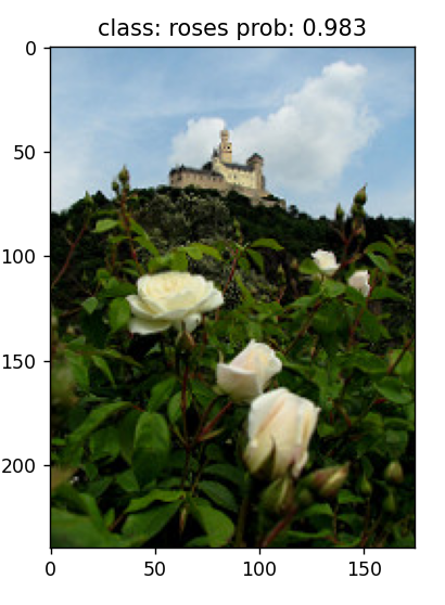
print_res = "class: {} prob: {:.3}".format(class_indict[str(predict_cla)], predict[predict_cla].numpy())
plt.title(print_res)
for i in range(len(predict)):
print("classes: {:10} prob: {:.3}".format(class_indict[str(i)], predict[i].numpy()))
plt.show()
if __name__ == '__main__':
img_path = "test.jpg"
weights_path = "./runs/ResNet34.pth"
nc = 5
main()

参考:
ResNet的几种典型网络结构 | Meringue's Blog
[学习笔记] ResNet,BN,以及迁移学习(附带TensorBoard可视化)_resnet bn-CSDN博客
|