深度学习 LSTM长短期记忆网络原理与Pytorch手写数字识别 |
您所在的位置:网站首页 › pytorch推荐算法 › 深度学习 LSTM长短期记忆网络原理与Pytorch手写数字识别 |
深度学习 LSTM长短期记忆网络原理与Pytorch手写数字识别
|
深度学习 LSTM长短期记忆网络原理与Pytorch手写数字识别
一、前言二、网络结构三、可解释性四、记忆主线五、遗忘门六、输入门七、输出门八、手写数字识别实战8.1 引入依赖库8.2 加载数据8.3 迭代训练8.4 数据验证
九、参考资料
一、前言
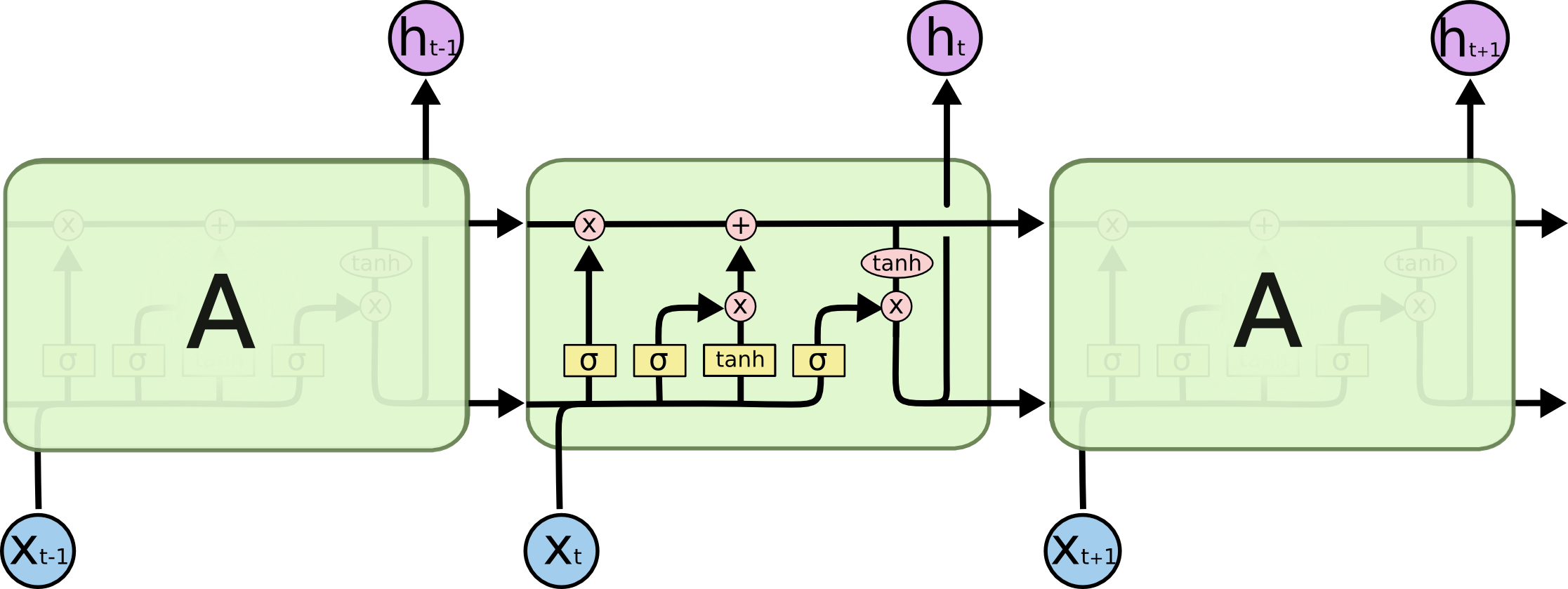
基本的RNN存在梯度消失和梯度爆炸问题,会忘记它在较长序列中以前看到的内容,只具有短时记忆。得到比较广泛应用的是LSTM(Long Short Term Memory)——长短期记忆网络,它在一定程度上解决了这两个问题。 二、网络结构我们来看一下LSTM网络的结构图: 为什么要这么设计LSTM网络呢?我们打个比方: 小明上次考了数学,留下的大部分是数学的知识记忆 C t − 1 C_{t-1} Ct−1;这次考生物,一些数学知识用不到,部分复杂的公式自然而然地被遗忘了 f t ⊙ C t − 1 f_t\odot{C}_{t-1} ft⊙Ct−1;复习生物知识一本书 C ~ t \tilde{C}_t C~t,大概记得八成 i t ⊙ C ~ t i_t\odot\tilde{C}_t it⊙C~t,那么当前的记忆 C t = f t ⊙ C t − 1 + i t ⊙ C ~ t C_t=f_t\odot{C}_{t-1}+i_t\odot\tilde{C}_t Ct=ft⊙Ct−1+it⊙C~t;考试时,成绩受到考题和当前记忆 C t C_t Ct的影响 h t = O t ⊙ tanh C t h_t=O_t\odot\tanh{C_t} ht=Ot⊙tanhCt。 注: ⊙ \odot ⊙是矩阵的点乘符号,即两个矩阵对应元素相乘 四、记忆主线
第一步,我们会遗忘部分原有的记忆。 第二步,我们会新增部分新的记忆。我们要确定,哪些新信息要保留到记忆细胞里。 C ~ t \tilde{C}_t C~t表示所有的输入信息,但我们不是所有的都记得, i t i_t it控制记忆程度, i t ⊙ C ~ t i_t\odot\tilde{C}_t it⊙C~t是本次输入所记住的信息。 遗忘后的记忆是 f t ⊙ C t − 1 f_t\odot{C}_{t-1} ft⊙Ct−1,输入新的记忆后, C t = f t ⊙ C t − 1 + i t ⊙ C ~ t C_t=f_t\odot{C}_{t-1}+i_t\odot\tilde{C}_t Ct=ft⊙Ct−1+it⊙C~t 七、输出门第三步,我们要根据现有记忆
C
t
C_t
Ct,输出我们需要的内容。 这就是LSTM网络的思想原理,接下来我们将用于手写数字识别实战。 八、手写数字识别实战 8.1 引入依赖库 import torch import torch.nn as nn from torchvision import datasets,transforms from torch.utils.data import DataLoader import matplotlib.pyplot as plt 8.2 加载数据 train_data = datasets.MNIST(root="./data",train=True,transform=transforms.ToTensor(),download=False) batch_size=64 train_loader = DataLoader(train_data,batch_size=batch_size,shuffle=True) test_data = datasets.MNIST(root="./data",train=False,transform=transforms.ToTensor(),download=False) test_x = test_data.data.type(torch.FloatTensor)[:2000]/255. #取2000个样本数据并将其缩放为0~1范围 test_y = test_data.targets[:2000] print(train_data.data.shape) torch.Size([60000, 28, 28]) 8.3 迭代训练 #迭代次数 epochs=1 #学习率 learning_rate=0.01 plt_epoch=[] plt_loss=[] class MyModel(nn.Module): def __init__(self): super().__init__() self.rnn = nn.LSTM( # LSTM 效果要比 nn.RNN() 好多了 input_size=28, # 图片每行的数据像素点 hidden_size=64, # rnn hidden unit num_layers=1, # 有几层 RNN layers batch_first=True, # input & output 会是以 batch size 为第一维度的特征集 e.g. (batch, time_step, input_size) ) self.out = nn.Linear(64, 10) # 输出层 def forward(self, x): # x shape (batch, time_step, input_size) # r_out shape (batch, time_step, output_size) # h_n shape (n_layers, batch, hidden_size) LSTM 有两个 hidden states, h_n 是分线, h_c 是主线 # h_c shape (n_layers, batch, hidden_size) r_out, (h_n, h_c) = self.rnn(x, None) # None 表示 hidden state 会用全0的 state # 选取最后一个时间点的 r_out 输出 # 这里 r_out[:, -1, :] 的值也是 h_n 的值 out = self.out(r_out[:, -1, :]) return out model = MyModel() #损失函数 cost=nn.CrossEntropyLoss() #迭代优化器 optmizer=torch.optim.Adam(model.parameters(),lr=learning_rate) for epoch in range(epochs): for step, (images, labels) in enumerate(train_loader): images=images.view(-1,28,28) #预测结果 output=model(images) #调用__call__函数 #计算损失值 loss=cost(output,labels) #在反向传播前先把梯度清零 optmizer.zero_grad() #反向传播,计算各参数对于损失loss的梯度 loss.backward() #根据刚刚反向传播得到的梯度更新模型参数 optmizer.step() plt_epoch.append(step+1) plt_loss.append(loss.item()) #打印损失值 if step % 50 == 0: pred_y = model(test_x) pred_y=pred_y.argmax(dim=1) #返回最大值的下标 print(f"step:{step},loss:{loss.item():.4f},accuracy: {(torch.sum(pred_y == test_y)/test_y.size()[0]) * 100:.2f}%") # 保存模型 torch.save(model, 'LSTM_Digits.pt') #绘制迭代次数与损失函数的关系 plt.plot(plt_epoch,plt_loss) step:0,loss:2.3081,accuracy: 8.75% step:50,loss:1.0913,accuracy: 59.40% step:100,loss:0.7879,accuracy: 70.30% step:150,loss:0.7618,accuracy: 73.75% step:200,loss:0.4271,accuracy: 86.70% step:250,loss:0.3963,accuracy: 90.65% step:300,loss:0.2965,accuracy: 91.85% step:350,loss:0.3396,accuracy: 94.15% step:400,loss:0.2283,accuracy: 92.30% step:450,loss:0.4932,accuracy: 94.05% step:500,loss:0.2487,accuracy: 93.25% step:550,loss:0.1460,accuracy: 94.20% step:600,loss:0.1908,accuracy: 94.70% step:650,loss:0.1521,accuracy: 92.35% step:700,loss:0.1530,accuracy: 94.80% step:750,loss:0.1192,accuracy: 94.65% step:800,loss:0.0478,accuracy: 95.30% step:850,loss:0.0535,accuracy: 95.70% step:900,loss:0.1174,accuracy: 95.45%
《如何从RNN起步,一步一步通俗理解LSTM》 《大白话讲解LSTM长短期记忆网络 如何缓解梯度消失,手把手公式推导反向传播》 《Understanding LSTM Networks》 《【Pytorch教程】:RNN 循环神经网络 (分类)》 |
 咱们放大看看,由于网上找不到清晰版的示例图,亲绘了一幅:
 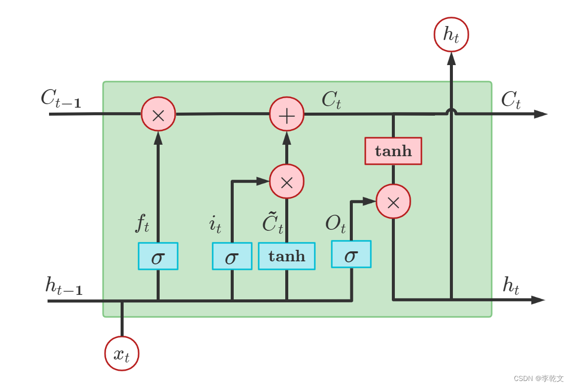 LSTM包含遗忘门、输入门、输出门。分别用于LSTM的三个步骤:旧记忆的遗忘、新记忆的输入、最终结果的输出。
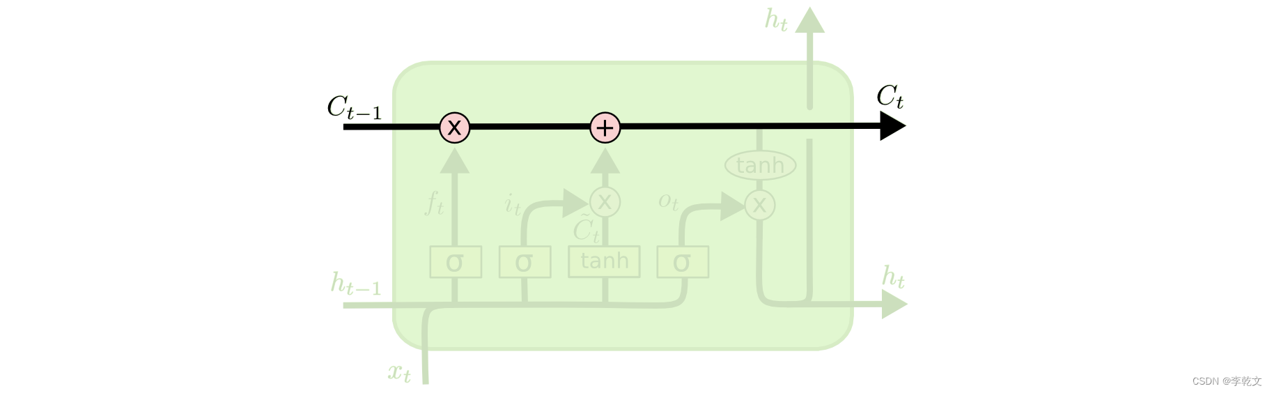 如上图所示,原有记忆是
C
t
−
1
C_{t-1}
Ct−1,经过遗忘(用矩阵参数进行点乘)、添加新记忆(加上新的记忆矩阵),当前最新的记忆就变成了
C
t
C_{t}
Ct,如此循环,不重要的记忆就会忘记、重要的记忆就会一直流传下去。
如上图所示,原有记忆是
C
t
−
1
C_{t-1}
Ct−1,经过遗忘(用矩阵参数进行点乘)、添加新记忆(加上新的记忆矩阵),当前最新的记忆就变成了
C
t
C_{t}
Ct,如此循环,不重要的记忆就会忘记、重要的记忆就会一直流传下去。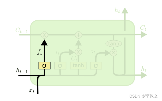 如上图所示,
f
t
=
σ
(
W
x
f
x
t
+
W
h
f
h
t
−
1
+
b
f
)
f_t=\sigma(W_{xf}x_t+W_{hf} h_{t-1}+b_f)
ft=σ(Wxfxt+Whfht−1+bf)
σ
\sigma
σ代表sigmoid函数。原有记忆是
C
t
−
1
C_{t-1}
Ct−1,遗忘后为
f
t
⊙
C
t
−
1
f_t\odot{C}_{t-1}
ft⊙Ct−1
如上图所示,
f
t
=
σ
(
W
x
f
x
t
+
W
h
f
h
t
−
1
+
b
f
)
f_t=\sigma(W_{xf}x_t+W_{hf} h_{t-1}+b_f)
ft=σ(Wxfxt+Whfht−1+bf)
σ
\sigma
σ代表sigmoid函数。原有记忆是
C
t
−
1
C_{t-1}
Ct−1,遗忘后为
f
t
⊙
C
t
−
1
f_t\odot{C}_{t-1}
ft⊙Ct−1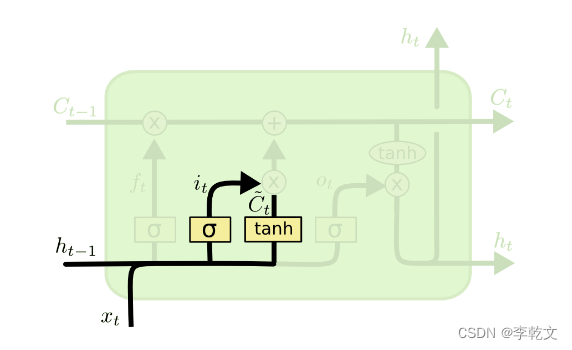 如上图所示,
C
~
t
=
t
a
n
h
(
W
x
c
x
t
+
W
h
c
h
t
−
1
+
b
c
)
i
t
=
σ
(
W
x
i
x
t
+
W
h
i
h
t
−
1
+
b
i
)
\begin{aligned} \tilde{C}_t&=tanh(W_{xc}x_t+W_{hc}h_{t-1} +b_c)\\ i_t&=\sigma(W_{xi}x_t+W_{hi} h_{t-1}+b_i) \end{aligned}
C~tit=tanh(Wxcxt+Whcht−1+bc)=σ(Wxixt+Whiht−1+bi)
如上图所示,
C
~
t
=
t
a
n
h
(
W
x
c
x
t
+
W
h
c
h
t
−
1
+
b
c
)
i
t
=
σ
(
W
x
i
x
t
+
W
h
i
h
t
−
1
+
b
i
)
\begin{aligned} \tilde{C}_t&=tanh(W_{xc}x_t+W_{hc}h_{t-1} +b_c)\\ i_t&=\sigma(W_{xi}x_t+W_{hi} h_{t-1}+b_i) \end{aligned}
C~tit=tanh(Wxcxt+Whcht−1+bc)=σ(Wxixt+Whiht−1+bi)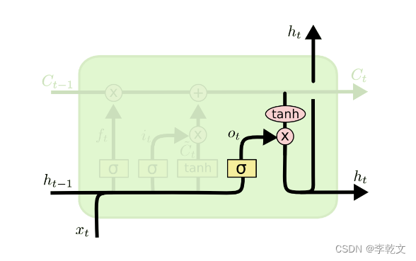 如上图所示,
O
t
=
σ
(
W
x
o
x
t
+
W
h
o
h
t
−
1
+
b
o
)
h
t
=
O
t
⊙
tanh
(
C
t
)
\begin{aligned} O_t&=\sigma(W_{xo}x_t+W_{ho} h_{t-1}+b_o)\\ h_t&=O_t\odot\tanh(C_t) \end{aligned}
Otht=σ(Wxoxt+Whoht−1+bo)=Ot⊙tanh(Ct)
如上图所示,
O
t
=
σ
(
W
x
o
x
t
+
W
h
o
h
t
−
1
+
b
o
)
h
t
=
O
t
⊙
tanh
(
C
t
)
\begin{aligned} O_t&=\sigma(W_{xo}x_t+W_{ho} h_{t-1}+b_o)\\ h_t&=O_t\odot\tanh(C_t) \end{aligned}
Otht=σ(Wxoxt+Whoht−1+bo)=Ot⊙tanh(Ct)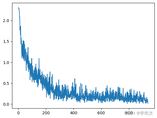
【本文地址】
今日新闻 |
推荐新闻 |