【PyTorch框架】 |
您所在的位置:网站首页 › pytorch指定多个gpu › 【PyTorch框架】 |
【PyTorch框架】
|
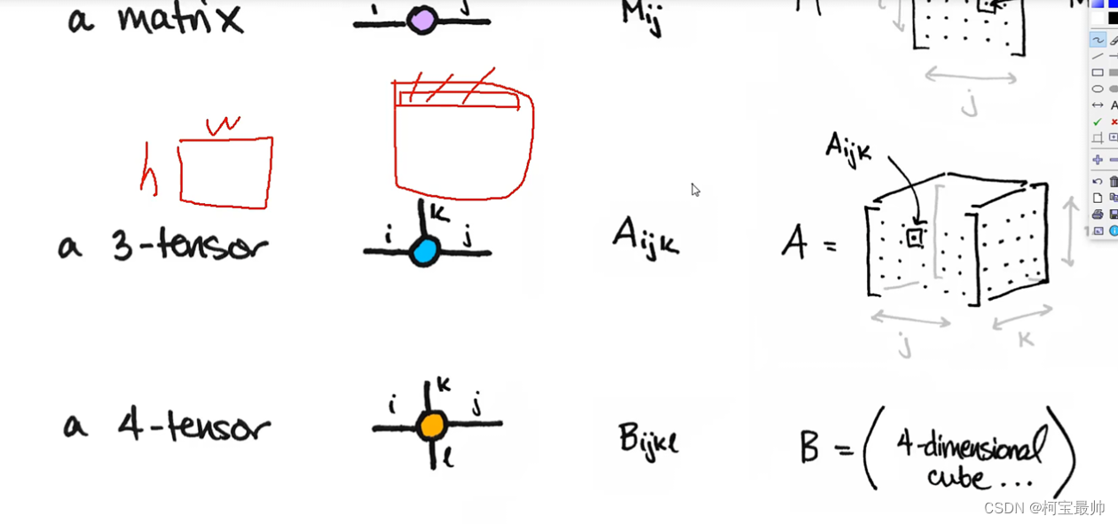
目录 一、引言 二、使用流程——最简单例子试手 三、分类任务——气温预测 总结: 一、引言Torch可以当作是能在GPU中计算的矩阵,就是ndarray的GPU版!TensorFlow和PyTorch可以说是当今最流行的框架!PyTorch用起来简单,好用!而TensoFlow用起来没那么自由!caffe比较老,不可处理文本数据,不推荐! 笔者用的时Pycharm的opencv环境! CPU版本:初学者,训练速度较慢!(到PyTorch官网去生成terminal命令如下) pip install torch torchvision torchaudio -i https://pypi.tuna.tsinghua.edu.cn/simple/ import torch print((torch.__version__))#查看Pytorch版本1.10.2+cpuGPU版本:项目!速度快!(也是到官网) 基本矩阵使用格式与numpy相似,只不过numpy得出的是ndarray的格式,而pytorch得到的矩阵式tensor的格式! x=torch.randn(6,6) y=x.view(36) z=x.view(-1,4) #-1表示自动计算另一个维度 print(x.size(),y.size(),z.size())框架最厉害的点之一就是可以帮我们把返向传播全部计算好(机器学习里的一个求导计算过程)!只需要在最后一层指定返向传播函数就可自动完成每一层求导过程。 tensor常见的形式:scalar、vector、matrix和n-dimensional tensor. scalar通常是一个数值;vector例如【-5.,2.,0.】通常指特征,例如词向量特征,某一维度的特征,是一组高维数据;多个特征组到一起形成一个矩阵matrix,通常都是高维的;通常处理图像时最低时3 tensor的,h,w,单个色彩通道这三维。 线性回归模型:(线性回归实际就是一个不加激活函数的全连接层) #构造一组输入数据x和其对应的标签y x_values=[i for i in range(11)] x_train=np.array(x_values,dtype = np.float32) x_train=x_train.reshape((-1,1)) #转置为列向量,-1表示行数自动计算 y_values=[3*i+4 for i in x_values] #线性关系y=3x+4 y_train=np.array(y_values,dtype = np.float32) y_train=x_train.reshape((-1,1)) #转置为列向量,-1表示行数自动计算①首先定义网络层: import torch import torch.nn as nn class LRM(nn.Module): def __init__(self,input_dim,output_dim): super(LRM,self).__init__() self.liner=nn.Linear(input_dim,output_dim)#全连接层,参数是输入输出的维度 def forward(self, x):#前向传播函数 out=self.liner(x) return out input_dim=1 output_dim=1 model=LRM(input_dim, output_dim) #调用线性回归函数,传入两个参数 print(model)
②指定好参数和损失函数: epochs=1000 #训练次数 learning_rate=0.01 #学习率 optimizer = torch.optim.SGD(model.parameters(), lr=learning_rate) #指定优化器,这里用SGD criterion=nn.MSELoss() #定义损失函数。分类任务用交叉熵;回归任务用MSELoss③训练模型: for epoch in range(epochs): epoch + 1 inputs=torch.from_numpy(x_train) #将x_train和y_train的ndarray格式转换为tensor格式,才可训练 labels=torch.from_numpy(y_train) optimizer.zero_grad() #梯度每一次迭代要清零,不然会累加 outputs=model(inputs) #前向传播 loss = criterion(outputs, labels) #计算损失 loss.backward() #返向传播 optimizer.step() #更新权重权重参数(会自动根据学习率和损失值完成更新)\ if epoch % 50 == 0: #为了观察内部变化,每隔50次打印下损失值 print('epoch{},loss{}'.format(epoch,loss.item()))
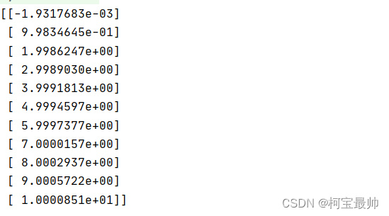
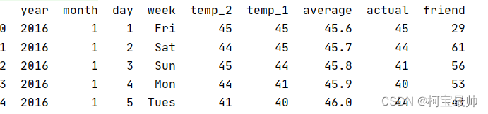
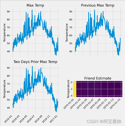
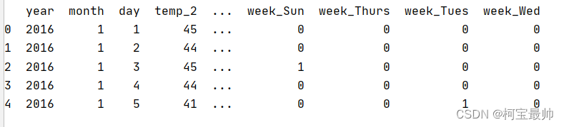
可以发现随着训练次数的增加,损失值一直减小到接近于0。 ④测试模型与预测结果: predicted=model(torch.from_numpy(x_train).requires_grad_()).data.numpy() #x_train转换为tensor传入model前向传播一次,最后再用data.numpy()转换为numpy的ndarray格式,便于打印显示 print(predicted) ⑤模型保存与读取 torch.save(model.state_dict(),'model.pkl') model.load_state_dict(torch.load('model.pkl')) 三、分类任务——气温预测①导入数据&数据前处理&查看数据分布&特征转换 import torch import pandas as pd import numpy as np import warnings warnings.filterwarnings("ignore") import matplotlib.pyplot as plt feasures = pd.read_csv("temps.csv") print(feasures.head())#打印几行查看下数据的样子
②构建网络模型&并训练(两种方法) 方法一: #构建网络模型——最麻烦的一种(基于底层运算) x = torch.tensor(input_features,dtype=float) #将x和y转换为tensor格式 y = torch.tensor(labels,dtype=float) weights = torch.randn((14,128),dtype=float, requires_grad=True) #权重参数初始化w1,b1,w2,b2。feature.shape是(348,14) biases = torch.randn(128,dtype=float, requires_grad=True) weights2 = torch.randn((128,1),dtype=float, requires_grad=True) biases2 = torch.randn(1,dtype=float, requires_grad=True) learning_rate = 0.001 #学习率 losses = [] for i in range(1000): #串起网络从前到后的计算流程,迭代1000次 hidden = x.mm(weights) + biases #计算隐层 hidden = torch.relu(hidden) #加入激活函数 predictions = hidden.mm(weights2) + biases2 #预测结果 loss = torch.mean((predictions - y) ** 2) #通计算损失 losses.append(loss.data.numpy()) if i % 100 == 0: print('loss:',loss) #每迭代100次打印一次损失值 loss.backward() #返向传播计算,等到grad梯度值 weights.data.add_(- learning_rate * weights.grad.data) #更新参数 biases.data.add_(- learning_rate * biases.grad.data) weights2.data.add_(- learning_rate * weights2.grad.data) biases2.data.add_(- learning_rate * biases2.grad.data) weights.grad.data.zero_() #每次迭代完记得将梯度清零 biases.grad.data.zero_() weights2.grad.data.zero_() biases2.grad.data.zero_()方法二: #更简单的构建网络模型方法(基于nn等模块里的功能函数) input_size = input_features.shape[1] hidden_size = 128 output_size = 1 batch_size = 16 my_nn = torch.nn.Sequential( torch.nn.Linear(input_size, hidden_size), torch.nn.Sigmoid(), torch.nn.Linear(hidden_size, output_size), ) cost = torch.nn.MSELoss(reduction='mean') optimizer = torch.optim.Adam(my_nn.parameters(), lr=0.001) #优化器,学习率会根据情况逐渐变化 #训练模型 losses = [] for i in range(1000): batch_loss = [] for start in range (0, len(input_features), batch_size): end = start + batch_size if start + batch_size < len(input_features) else len(input_features) xx = torch.tensor(input_features[start: end],dtype=torch.float, requires_grad=True) yy = torch.tensor(labels[start: end],dtype=torch.float, requires_grad=True) predictions = my_nn(xx) #预测 loss = cost(predictions, yy) #损失 optimizer.zero_grad() #梯度清零 loss.backward(retain_graph=True) #返向传播 optimizer.step() batch_loss.append(loss.data.numpy()) if i % 100 == 0:#打印损失 losses.append(np.mean(batch_loss)) print(i,np.mean(batch_loss))③预测训练结果 #预测训练结果 x = torch.tensor(input_features, dtype=torch.float) predict = my_nn(x).data.numpy() #转换日期格式 dates = [str(int(year)) + '-' + str(int(month)) + '-' + str(int(day)) for year,month,day in zip(years,months,days)] dates = [datetime.datetime.strptime(date,'%Y-%m-%d') for date in dates] #创建表格来存日期和其对应的标签数值 true_data = pd.DataFrame(data={'date': dates, 'actual': labels}) #再创建表格来存日期和其对应的模型预测值 years = feasures[:,feasure_list.index('year')] months = feasures[:,feasure_list.index('month')] days = feasures[:,feasure_list.index('day')] test_dates =[str(int(year)) + '-' + str(int(month)) + '-' + str(int(day)) for year,month,day in zip(years,months,days)] test_dates = [datetime.datetime.strptime(date,'%Y-%m-%d') for date in test_dates] predictions_data = pd.DataFrame(data={'dates': test_dates, 'prediction': predict.reshape(-1)}) #画图显示 plt.plot(true_data['date'], true_data['actual'], 'b-', label = 'actual')#真实值 plt.plot(predictions_data['date'], predictions_data['prediction'], 'ro', label = 'prediction')#预测值 plt.xticks(rotation='60') plt.legend() 总结:由于是初学者可能很多地方没有总结完全或者有误,后续深入学习后会不断回来该删,也欢迎各位朋友指正!
|


【本文地址】
今日新闻 |
推荐新闻 |