|
BP 算法是一个迭代算法,它的基本思想为:(1) 先计算每一层的状态和激活值,直到最后一层(即信号是前向传播的);(2) 计算每一层的误差,误差的计算过程是从最后一层向前推进的(这就是反向传播算法名字的由来);(3) 更新参数(目标是误差变小),迭代前面两个步骤,直到满足停止准则(比如相邻两次迭代的误差的差别很小)。 下面用图片的形式展示其推到过程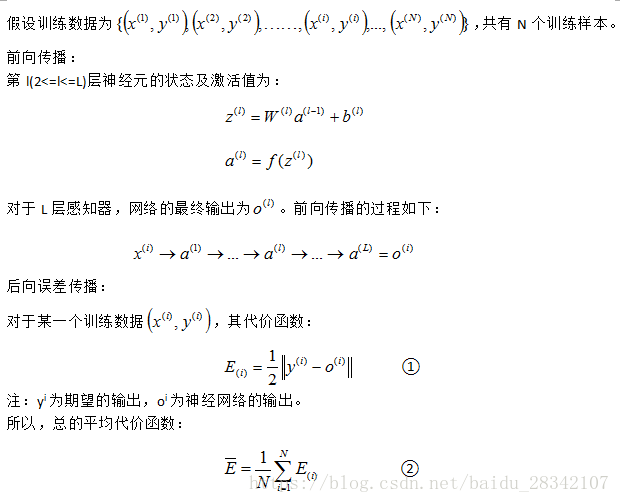 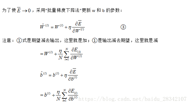 数据集:数据集采用Sort_1000pics数据集。数据集包含1000张图片,总共分为10类。分别是人(0),沙滩(1),建筑(2),大卡车(3),恐龙(4),大象(5),花朵(6),马(7),山峰(8),食品(9)十类,每类100张,(数据集可以到网上下载)。注意网上下载的数据集是一个整体,需要自己手动将图片进行整理分类,方便python进行读取操作,参考和参考进行数据集处理。 数据集:数据集采用Sort_1000pics数据集。数据集包含1000张图片,总共分为10类。分别是人(0),沙滩(1),建筑(2),大卡车(3),恐龙(4),大象(5),花朵(6),马(7),山峰(8),食品(9)十类,每类100张,(数据集可以到网上下载)。注意网上下载的数据集是一个整体,需要自己手动将图片进行整理分类,方便python进行读取操作,参考和参考进行数据集处理。
import datetime
starttime = datetime.datetime.now()
import numpy as np
from sklearn.cross_validation import train_test_split
from sklearn.metrics import confusion_matrix, classification_report
import os
import cv2
X = []
Y = []
for i in range(0, 10):
#遍历文件夹,读取图片
for f in os.listdir("./photo/%s" % i):
#打开一张图片并灰度化
Images = cv2.imread("./photo/%s/%s" % (i, f))
image=cv2.resize(Images,(256,256),interpolation=cv2.INTER_CUBIC)
hist = cv2.calcHist([image], [0,1], None, [256,256], [0.0,255.0,0.0,255.0])
X.append((hist/255).flatten())
Y.append(i)
X = np.array(X)
Y = np.array(Y)
#切分训练集和测试集
X_train, X_test, y_train, y_test = train_test_split(X, Y, test_size=0.3, random_state=1)
from sklearn.preprocessing import LabelBinarizer
import random
def logistic(x):
return 1 / (1 + np.exp(-x))
def logistic_derivative(x):
return logistic(x) * (1 - logistic(x))
class NeuralNetwork:
def predict(self, x):
for b, w in zip(self.biases, self.weights):
# 计算权重相加再加上偏向的结果
z = np.dot(x, w) + b
# 计算输出值
x = self.activation(z)
return self.classes_[np.argmax(x, axis=1)]
class BP(NeuralNetwork):
def __init__(self,layers,batch):
self.layers = layers
self.batch = batch
self.activation = logistic
self.activation_deriv = logistic_derivative
self.num_layers = len(layers)
self.biases = [np.random.randn(x) for x in layers[1:]]
self.weights = [np.random.randn(x, y) for x, y in zip(layers[:-1], layers[1:])]
def fit(self, X, y, learning_rate=0.1, epochs=1):
labelbin = LabelBinarizer()
y = labelbin.fit_transform(y)
self.classes_ = labelbin.classes_
training_data = [(x,y) for x, y in zip(X, y)]
n = len(training_data)
for k in range(epochs):
#每次迭代都循环一次训练
# 搅乱训练集,让其排序顺序发生变化
random.shuffle(training_data)
batches = [training_data[k:k+self.batch] for k in range(0, n, self.batch)]
#批量梯度下降
for mini_batch in batches:
x = []
y = []
for a,b in mini_batch:
x.append(a)
y.append(b)
activations = [np.array(x)]
#向前一层一层的走
for b, w in zip(self.biases, self.weights):
#计算激活函数的参数,计算公式:权重.dot(输入)+偏向
z = np.dot(activations[-1],w)+b
#计算输出值
output = self.activation(z)
#将本次输出放进输入列表,后面更新权重的时候备用
activations.append(output)
#计算误差值
error = activations[-1]-np.array(y)
#计算输出层误差率
deltas = [error * self.activation_deriv(activations[-1])]
#循环计算隐藏层的误差率,从倒数第2层开始
for l in range(self.num_layers-2, 0, -1):
deltas.append(self.activation_deriv(activations[l]) * np.dot(deltas[-1],self.weights[l].T))
#将各层误差率顺序颠倒,准备逐层更新权重和偏向
deltas.reverse()
#更新权重和偏向
for j in range(self.num_layers-1):
# 权重的增长量,计算公式,增长量 = 学习率 * (错误率.dot(输出值)),单个训练数据的误差
delta = learning_rate/self.batch*((np.atleast_2d(activations[j].sum(axis=0)).T).dot(np.atleast_2d(deltas[j].sum(axis=0))))
#更新权重
self.weights[j] -= delta
#偏向增加量,计算公式:学习率 * 错误率
delta = learning_rate/self.batch * deltas[j].sum(axis=0)
#更新偏向
self.biases[j] -= delta
return self
clf0 = BP([X_train.shape[1],10],10).fit(X_train,y_train,epochs=100)
predictions_labels = clf0.predict(X_test)
print(confusion_matrix(y_test, predictions_labels))
print (classification_report(y_test, predictions_labels))
endtime = datetime.datetime.now()
print (endtime - starttime)
实验结果为:
[[19 0 1 0 0 2 1 1 6 1]
[ 2 10 6 1 0 3 0 1 7 1]
[ 3 1 12 1 0 3 1 0 3 2]
[ 1 0 0 21 0 0 1 0 3 3]
[ 0 1 1 0 29 0 0 1 0 0]
[ 1 7 1 0 1 17 1 2 2 2]
[ 2 0 1 0 0 0 24 0 1 2]
[ 2 0 0 0 0 1 0 21 0 2]
[ 2 1 2 2 0 2 0 0 20 2]
[ 0 1 3 2 2 1 2 2 1 16]]
precision recall f1-score support
0 0.59 0.61 0.60 31
1 0.48 0.32 0.38 31
2 0.44 0.46 0.45 26
3 0.78 0.72 0.75 29
4 0.91 0.91 0.91 32
5 0.59 0.50 0.54 34
6 0.80 0.80 0.80 30
7 0.75 0.81 0.78 26
8 0.47 0.65 0.54 31
9 0.52 0.53 0.52 30
avg / total 0.63 0.63 0.63 300
0:01:14.663123
因为权值和阈值每次都是随机初始化的,所以每次运行结果就会不一样。读者可以更改w和b的值,将其调整到更佳的状态。
参考:https://www.jianshu.com/p/c7e642877b0e(梯度下降法及其实现) 参考:https://www.leiphone.com/news/201705/TMsNCqjpOIfN3Bjr.html 参考:https://www.k2zone.cn/?p=1110
|