一文通俗入门·脉冲神经网络(SNN)·第三代神经网络 |
您所在的位置:网站首页 › pnn神经网络程序训练 › 一文通俗入门·脉冲神经网络(SNN)·第三代神经网络 |
一文通俗入门·脉冲神经网络(SNN)·第三代神经网络
|
原创文章,转载请注明出处:https://blog.csdn.net/weixin_37864449/article/details/126772830?spm=1001.2014.3001.5502
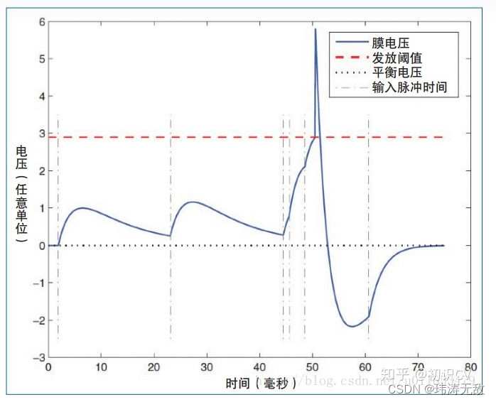
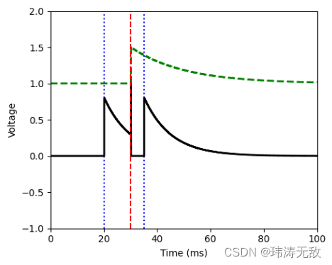
如上动态图所示,脉冲网络由脉冲神经元连接而成,脉冲神经元输入为脉冲,输出也是脉冲,脉冲神经元内部有电动势v,v在没有接收到任何输入时会随着时间指数衰减到某个稳定的电动势(平衡电压),而某一时刻接收到输入脉冲时电动势会增加某个值,当电动势增加的速度快过衰减的速度时(如频繁有脉冲输入),神经元内部的电动势会越来越大,直到达到某个发放阈值后该脉冲神经元会发放脉冲,此后脉冲神经元电动势迅速置为静息电动势,电动势变化过程如下图二所示。电动势变化的规律又称为神经电位动力学。
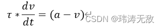
图二 神经元膜电压变化 一、脉冲神经元模型脉冲神经元电位动力学数学模型最简单常用的是漏电积分-放电(leaky integrate-and-fire ( LIF ))模型,这个模型工作过程与生物神经元充电、漏电、放电过程类似,更精确的描述生物神经动力学模型是Hodgkin-huxley模型,但该模型微分方程复杂难以直观理解,虽然Hodgkin-huxley模型更精确描述了生物神经元电位动力学变化过程,但有观点认为该模型对数据拟合能力没有LIF模型好(https://www.youtube.com/watch?v=GTXTQ_sOxak 25:24),总而言之,LIF是基于生物神经元动力学特性简化后的数学模型,简单好用,下面详细讨论LIF模型。 我们知道,每个脉冲神经元内部有电压v,当没有接收到任何脉冲输入时,电压v会随着时间指数稳定到平衡电压
求解这个微分方程,可以得到:
这里 上面是连续电压
故微分方程的离散形式为:
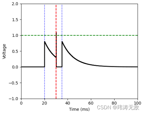
另外,当某个时刻神经元接收到一个脉冲输入时,则要累积该脉冲到电压中,最简单的方式是让当前的电压加上某个值,通常这个值跟连接该输入脉冲的突触权重有关,电压更新过程为: 神经元内部有一个发放阈值 为更好的理解LIF模型控制的神经元膜电压变化,下面附上由for循环实现的python代码: import numpy as np import matplotlib.pyplot as plt fig = plt.figure(figsize=(5, 4)) ax = plt.subplot(111) # Function that runs the simulation # tau: time constant (in ms) # t0, t1, t2: time of three input spikes # w: input synapse weight # threshold: threshold value to produce a spike # reset: reset value after a spike def LIF(tau=10, t0=20, t1=30, t2=35, w=0.8, threshold=1.0, reset=0.0): # Spike times, keep sorted because it's more efficient to pop the last value off the list times = [t0, t1, t2] times.sort(reverse=True) # set some default parameters duration = 100 # total time in ms dt = 0.1 # timestep in ms alpha = np.exp(-dt / tau) # this is the factor by which V decays each time step V_rec = [] # list to record membrane potentials V = 0.0 # initial membrane potential T = np.arange(np.round(duration / dt)) * dt # array of times spikes = [] # list to store spike times # run the simulation # plot everything (T is repeated because we record V twice per loop) ax.clear() for t in times: ax.axvline(t, ls=':', c='b') for t in T: V_rec.append(V) # record V *= alpha # integrate equations if times and t > times[-1]: # if there has been an input spike V +=w times.pop() # remove that spike from list V_rec.append(V) # record V before the reset so we can see the spike if V > threshold: # if there should be an output spike V = reset spikes.append(t) ax.plot(np.repeat(T, 2), V_rec, '-k', lw=2) for t in spikes: ax.axvline(t, ls='--', c='r') ax.axhline(threshold, ls='--', c='g') ax.set_xlim(0, duration) ax.set_ylim(-1, 2) ax.set_xlabel('Time (ms)') ax.set_ylabel('Voltage') plt.tight_layout() plt.show() LIF()运行结果为:
绿色虚线表示发放阈值 更复杂一些,我们可以让发放阈值也能发生变化,下面代码演示了当神经元发放脉冲时,发放阈值会增加某个值,且发放阈值动力学模型也是LIF模型。 import numpy as np import matplotlib.pyplot as plt fig = plt.figure(figsize=(5, 4)) ax = plt.subplot(111) # Function that runs the simulation # tau: time constant (in ms) # t0, t1, t2: time of three input spikes # w: input synapse weight # threshold: threshold value to produce a spike # reset: reset value after a spike def LIF2(tau=10, taut=20, t0=20, t1=30, t2=35, w=0.8, threshold=1.0, dthreshold=0.5, reset=0.0): # Spike times, keep sorted because it's more efficient to pop the last value off the list times = [t0, t1, t2] times.sort(reverse=True) # set some default parameters duration = 100 # total time in ms dt = 0.1 # timestep in ms alpha = np.exp(-dt/tau) # this is the factor by which V decays each time step beta = np.exp(-dt/taut) # this is the factor by which Vt decays each time step V_rec = [] # list to record membrane potentials Vt_rec = [] # list to record threshold values V = 0.0 # initial membrane potential Vt = threshold T = np.arange(np.round(duration/dt))*dt # array of times spikes = [] # list to store spike times # clear the axis and plot the spike times ax.clear() for t in times: ax.axvline(t, ls=':', c='b') # run the simulation for t in T: V_rec.append(V) # record Vt_rec.append(Vt) V *= alpha # integrate equations Vt = (Vt-threshold)*beta+threshold if times and t>times[-1]: # if there has been an input spike V += w times.pop() # remove that spike from list V_rec.append(V) # record V before the reset so we can see the spike Vt_rec.append(Vt) if V>Vt: # if there should be an output spike V = reset Vt += dthreshold spikes.append(t) # plot everything (T is repeated because we record V twice per loop) ax.plot(np.repeat(T, 2), V_rec, '-k', lw=2) ax.plot(np.repeat(T, 2), Vt_rec, '--g', lw=2) for t in spikes: ax.axvline(t, ls='--', c='r') ax.set_xlim(0, duration) ax.set_ylim(-1, 2) ax.set_xlabel('Time (ms)') ax.set_ylabel('Voltage') plt.tight_layout() plt.show() #display(fig) LIF2()运行结果为:
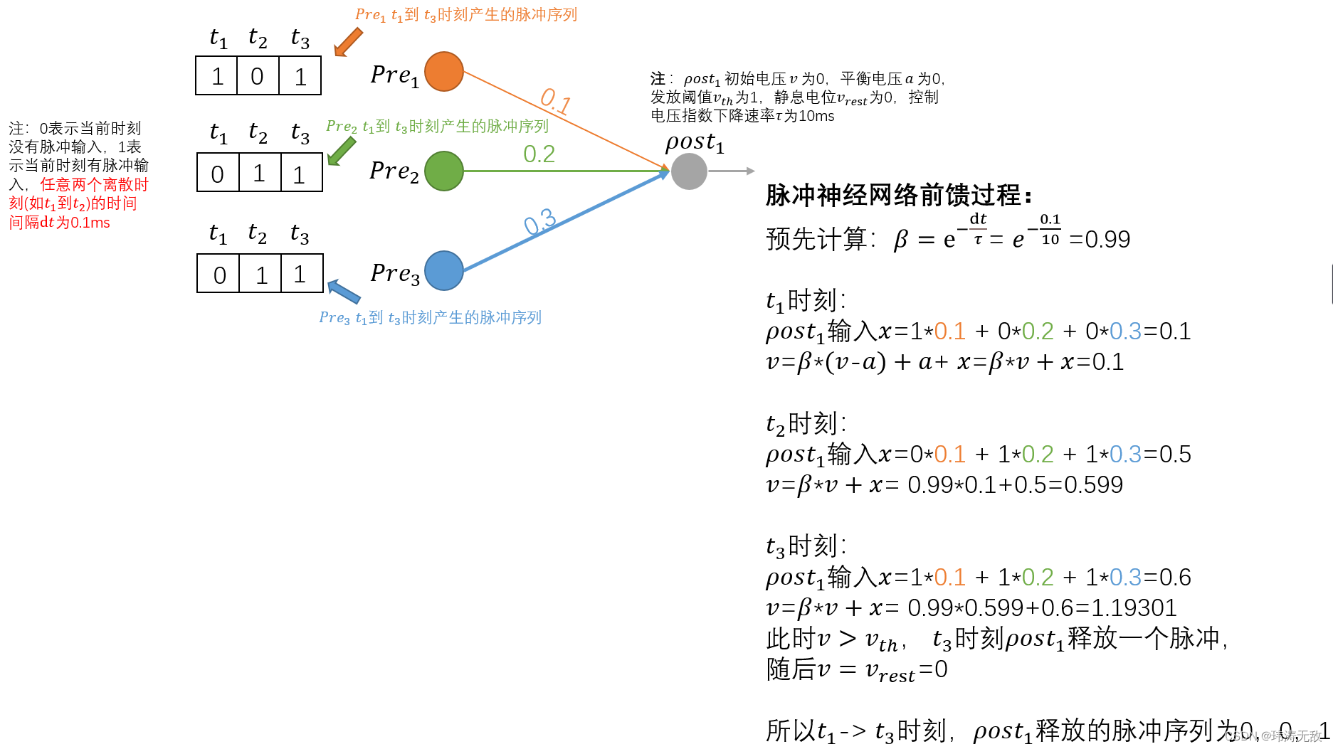
有了上面的知识后,我们来简单模拟一下脉冲神经网络前向传播的过程:
前面我们知道了脉冲神经元内部的电动力学特性及其方程,接下来我们来学习如何更新脉冲神经网络的连接权重,区别于传统的梯度下降方法,脉冲神经网络通常使用的是更具生物学特性的STDP(spike timing dependent plasticity)学习策略。在解释STDP之前,我们先来看看一些概念:
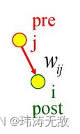
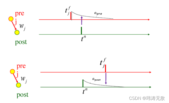
如上图所示,脉冲神经元连接有前突触和后突触之分,索引j 神经元称为前突触,若神经元j产生了一个脉冲,则称神经元j产生了一个突触前脉冲,索引i 神经元称为后突触,同理神经元i产生的脉冲称为突触后脉冲。j与i的连接权重为
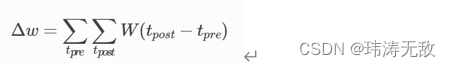
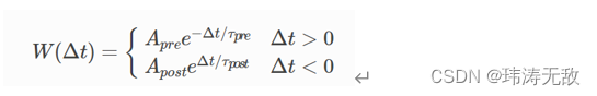
根据上面的定义,STDP更新权重的公式可写成:
也就是说,突触权重
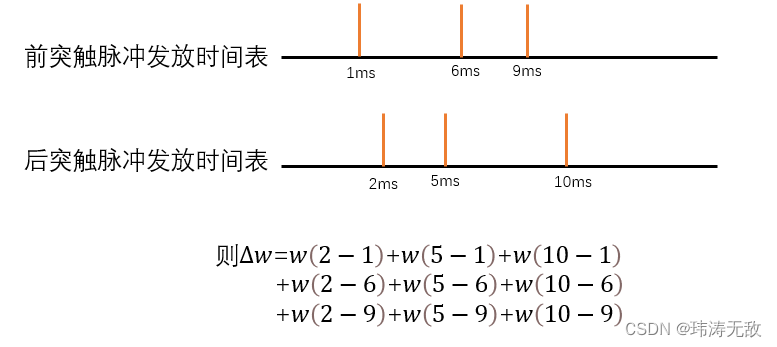
举个例子:
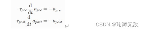
然而使用该定义需要事先知道前突触脉冲和后突触脉冲一段时间内各自发放脉冲的时间表,因此直接使用这个方程更新权重将非常低效,因为我们必须对每个神经元先记录好它的脉冲发放时间表,然后对所有尖峰对时间差求和。这在生物学上也是不现实的,因为神经元无法记住之前的所有尖峰时间。事实证明,有一种更有效、生理上更合理的方法可以达到同样的效果,该方法可以在突触前脉冲发放或突触后脉冲发放就立刻更新权重。 我们先定义两个新变量
痕迹变化由LIF模型控制:
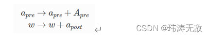
当发放突触前脉冲时,会更新突触前活动痕迹变量并根据规则修改权重w:
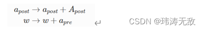
同理当突触后脉冲发放时:
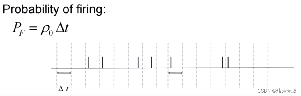
这个更新公式可以理解为:当突触前脉冲到达了,突触后脉冲痕迹还未衰减到0,说明突触后脉冲是比突触前脉冲早到达的,所以权重应该削弱,削弱量为 最后,我们看一下泊松脉冲编码。由于脉冲神经网络接收的是脉冲信号,所以需要对初始输入数据进行脉冲编码,其中输入数据脉冲编码一个比较常用的方式是泊松脉冲编码,更详细的泊松脉冲编码讲解可参考:https://www.youtube.com/watch?v=4r_gc4vf8eE 。
泊松脉冲编码首先需要设置脉冲速率ρ0 ,ρ0 可以是常数,也可以是时间函数。编码过程可描述为:取时间间隔为Δt ,则每个时间间隔脉冲发放的概率为pF=ρ0*Δt ,电脑在每个时间间隔生成一个(0,1)范围内均匀分布的随机数,随机数小于ρ0*Δt 则在该时间间隔内产生一个脉冲。 泊松脉冲编码可以这样应用:把输入时间序列值看成脉冲速率ρ0 ,如t1时刻输入为a, t2时刻输入为b,t3时刻输入为c,若t1时刻0-1随机数大于或等于a*Δt ,则t1时刻神经元不发放脉冲,t2时刻0-1随机数小于b*Δt ,则t2时刻神经元发放脉冲,t3时刻0-1随机数大于或等于c*Δt ,则t3时刻神经元不发放脉冲,所以a,b,c编码后的脉冲序列为无脉冲,脉冲,无脉冲。 最后,推荐一个可以用来学习脉冲神经网络特性的编程工具包:brian2python安装方式:pip install brian2 教程:Introduction to Brian part 1: Neurons — Brian 2 2.5.1 documentation |

【本文地址】
今日新闻 |
推荐新闻 |