MATLAB |
您所在的位置:网站首页 › matlab怎么画电路 › MATLAB |
MATLAB
|
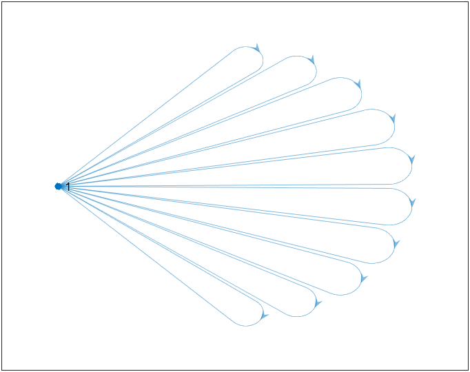
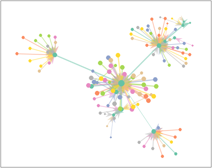
一篇超超超长,超超超全面网络图绘制教程,本篇基本能讲清楚所有绘制要点,当然图论与网络优化的算法一篇不可能完全讲清楚,未来如果看的人多可以适当更新,同时做部分网络图绘图复刻。 以下是本篇绘图实验效果:
可以通过 graph 函数创建无向图,通过 digraph 创建有向图,其中网络创建可以使用起始终止点数组、邻接矩阵、EdgeTable等几种方式。 1.1 起始终止点数组不点名布局时它会自动选择比较清晰的布局方式,怎么改布局之后再说,以下两个图连线情况都是一样的,不过有向图为了更好展示方向箭头自动用了不同的布局。 s=[1 1 1 1 1 1 1 9 9 9 9 9 9 9]; t=[2 3 4 5 6 7 8 2 3 4 5 6 7 8]; G=graph(s,t); plot(G)
无向图邻接矩阵必须是对称的,但是可以通过设置lower或upper属性使用下三角或上三角矩阵。 s=[1 1 1 1 1 1 1 9 9 9 9 9 9 9]; t=[2 3 4 5 6 7 8 2 3 4 5 6 7 8]; A=zeros(max(s)); for i=1:length(s) A(s(i),t(i))=1; A(t(i),s(i))=1; end % A = [0 1 1 1 1 1 1 1 0 % 1 0 0 0 0 0 0 0 1 % 1 0 0 0 0 0 0 0 1 % 1 0 0 0 0 0 0 0 1 % 1 0 0 0 0 0 0 0 1 % 1 0 0 0 0 0 0 0 1 % 1 0 0 0 0 0 0 0 1 % 1 0 0 0 0 0 0 0 1 % 0 1 1 1 1 1 1 1 0]; G=graph(A); plot(G)通过设置upper属性使用上三角矩阵: s=[1 1 1 1 1 1 1 9 9 9 9 9 9 9]; t=[2 3 4 5 6 7 8 2 3 4 5 6 7 8]; A=zeros(max(s)); for i=1:length(s) A(min(s(i),t(i)),max(s(i),t(i)))=1; end % A = [0 1 1 1 1 1 1 1 0 % 0 0 0 0 0 0 0 0 1 % 0 0 0 0 0 0 0 0 1 % 0 0 0 0 0 0 0 0 1 % 0 0 0 0 0 0 0 0 1 % 0 0 0 0 0 0 0 0 1 % 0 0 0 0 0 0 0 0 1 % 0 0 0 0 0 0 0 0 1 % 0 0 0 0 0 0 0 0 0]; G=graph(A,'upper'); plot(G)
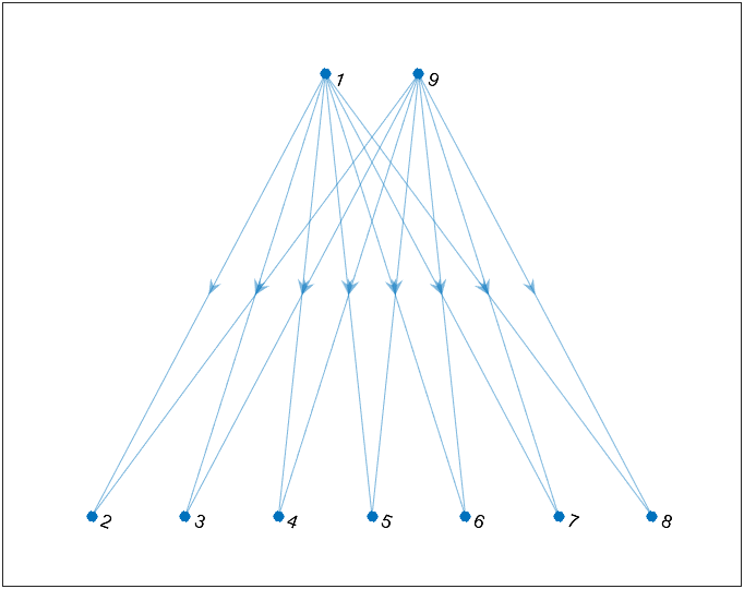
有向图第 i 行第 j 列有数值就说明有从 i 流向 j 的箭头。此处不要求对称矩阵啦。 s=[1 1 1 1 1 1 1 9 9 9 9 9 9 9]; t=[2 3 4 5 6 7 8 2 3 4 5 6 7 8]; A=zeros(max(s)); for i=1:length(s) A(s(i),t(i))=1; end G=digraph(A); plot(G,'Layout','layered')
如果矩阵是对称的就说明流动是双向的: s=[1 1 1 1 1 1 1 9 9 9 9 9 9 9]; t=[2 3 4 5 6 7 8 2 3 4 5 6 7 8]; A=zeros(max(s)); for i=1:length(s) A(s(i),t(i))=1; A(t(i),s(i))=1; end G=digraph(A); plot(G,'Layout','layered')
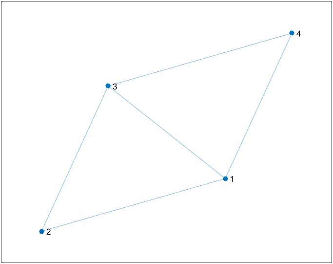
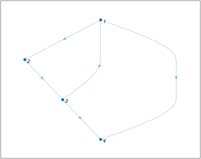
先展示一下最简单的啥都没有的网络图,之后会给出边表中增添权重,增添标签名称啥的方法的! s=[1 1 1 2 3]; t=[2 3 4 3 4]; EdgeTable=table([s' t'],'VariableNames',{'EndNodes'}); % EdgeTable = % % 5×1 table % EndNodes % ________ % 1 2 % 1 3 % 1 4 % 2 3 % 3 4 G=graph(EdgeTable); plot(G)
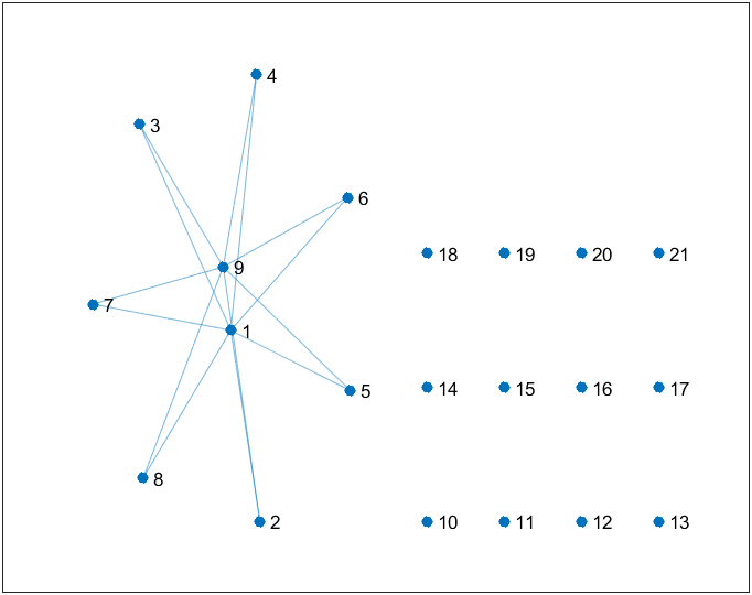
通过如下方式可以设置节点总数: s=[1 1 1 1 1 1 1 9 9 9 9 9 9 9]; t=[2 3 4 5 6 7 8 2 3 4 5 6 7 8]; G=graph(s,t,[],21); plot(G)
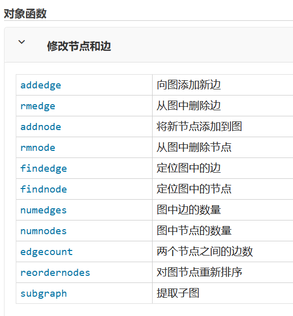
实际上是使用,以下的 addnode 及 addedge 函数实现的:
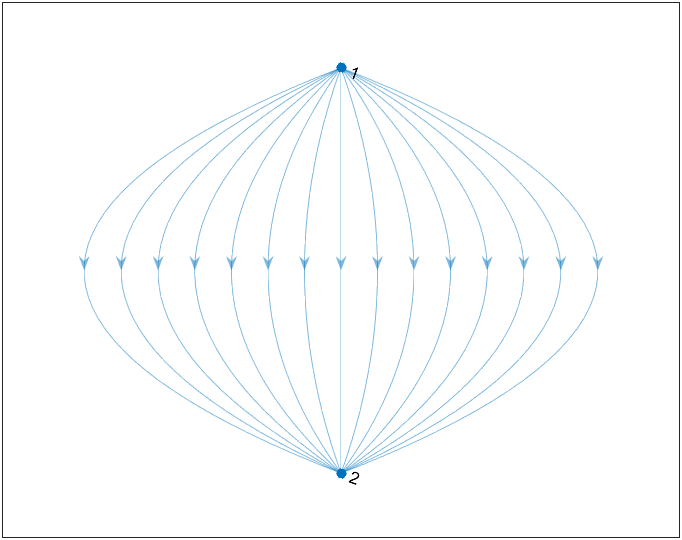
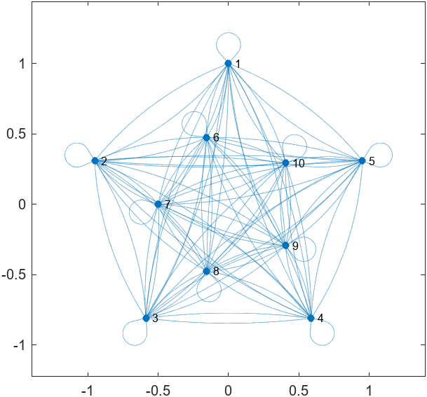
两点之间不仅仅只能有两条边。 s=ones(1,15); t=2.*ones(1,15); G=digraph(s,t); plot(G)
自己到自己的边也是可以有且能有很多条的: s=ones(1,10); t=ones(1,10); G=digraph(s,t); plot(G)
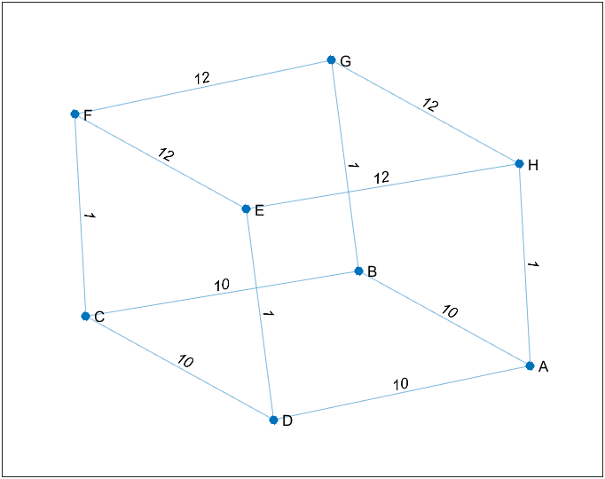
对于由起始终止点数组创建的图: s=[1 1 1 2 2 3 3 4 5 5 6 7]; t=[2 4 8 3 7 4 6 5 6 8 7 8]; weights=[10 10 1 10 1 10 1 1 12 12 12 12]; names={'A' 'B' 'C' 'D' 'E' 'F' 'G' 'H'}; G=graph(s,t,weights,names); plot(G,'EdgeLabel',weights)对于边表创建时增添权重及节点名称: s=[1 1 1 2 2 3 3 4 5 5 6 7]; t=[2 4 8 3 7 4 6 5 6 8 7 8]; weights=[10 10 1 10 1 10 1 1 12 12 12 12]; names={'A' 'B' 'C' 'D' 'E' 'F' 'G' 'H'}; EdgeTable=table([s' t'],weights','VariableNames',{'EndNodes' 'Weights'}); NodeTable=table(names','VariableNames',{'Name'}); % EdgeTable = % % 12×2 table % EndNodes Weights % ________ _______ % 1 2 10 % 1 4 10 % 1 8 1 % ... ... ... % 6 7 12 % 7 8 12 G=graph(EdgeTable,NodeTable); plot(G,'EdgeLabel',weights)
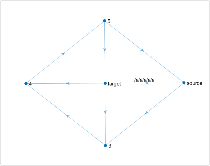
当然可以仅仅为部分添加: s=[1 1 2 2 3 4 5 5]; t=[2 3 3 4 4 5 1 2]; G=digraph(s,t); h=plot(G); labelnode(h,[1 2],{'source' 'target'}) labeledge(h,1,2,'lalalalala')
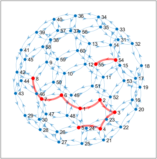
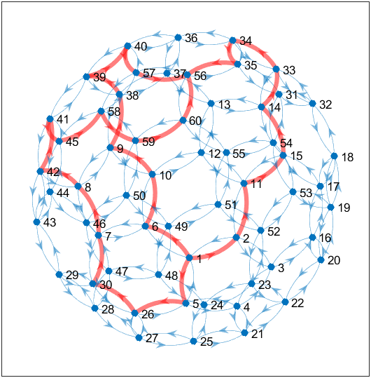
比如说把如下点和边标为红色: G=digraph(bucky); h=plot(G); highlight(h,[8,7,6,1,2,3,4,5,54,55],'NodeColor','red','MarkerSize',5) highlight(h,[8,7,6,1,2,3,4,5,54,55],'EdgeColor','red','LineWidth',3) axis tight equal
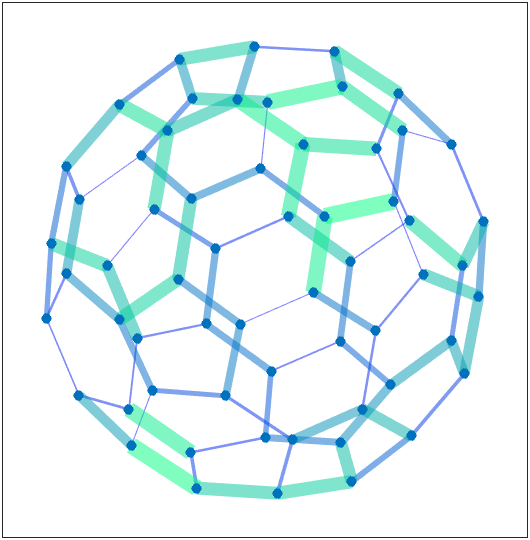
但其实最好用边表来增添高亮,很多图论与网络优化官方函数的返回值都是边表: G=digraph(bucky); h=plot(G); [mf,GF]=maxflow(G,1,56); highlight(h,GF,'EdgeColor','red','LineWidth',3) axis tight equal
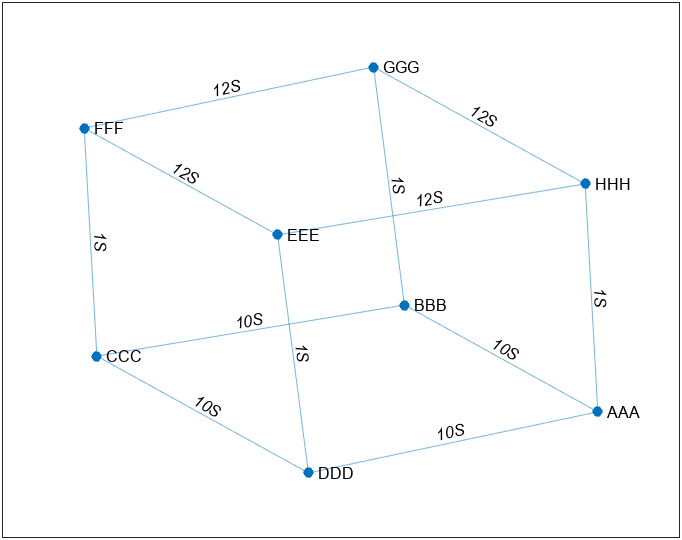
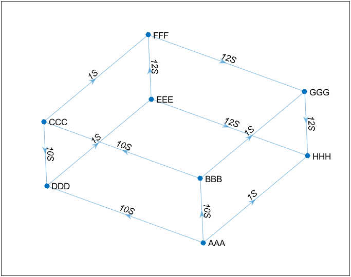
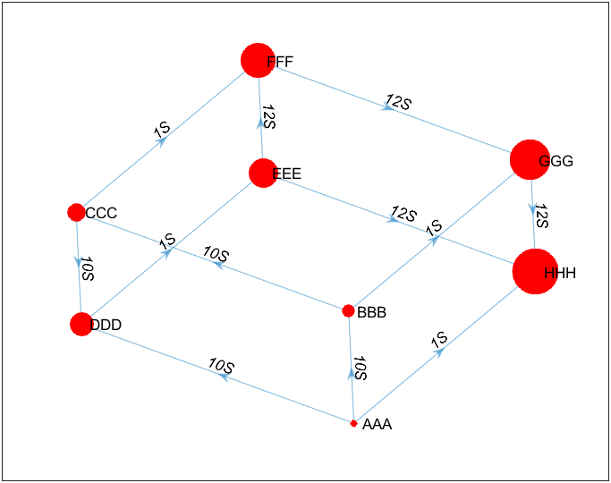
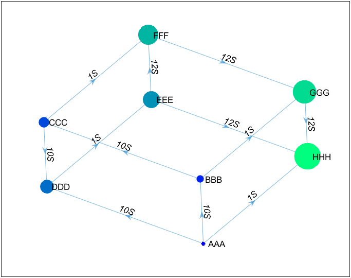
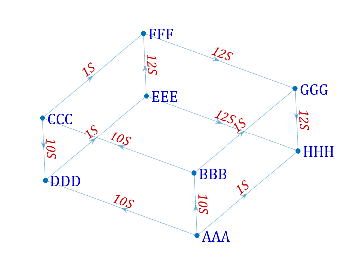
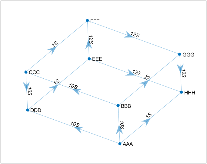
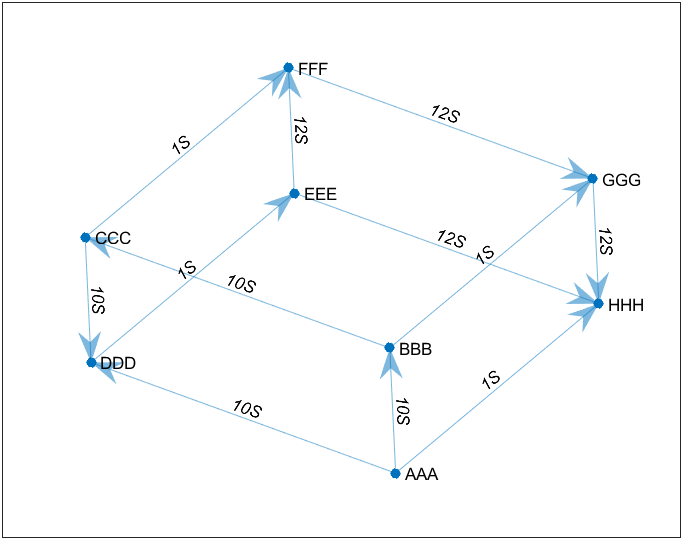
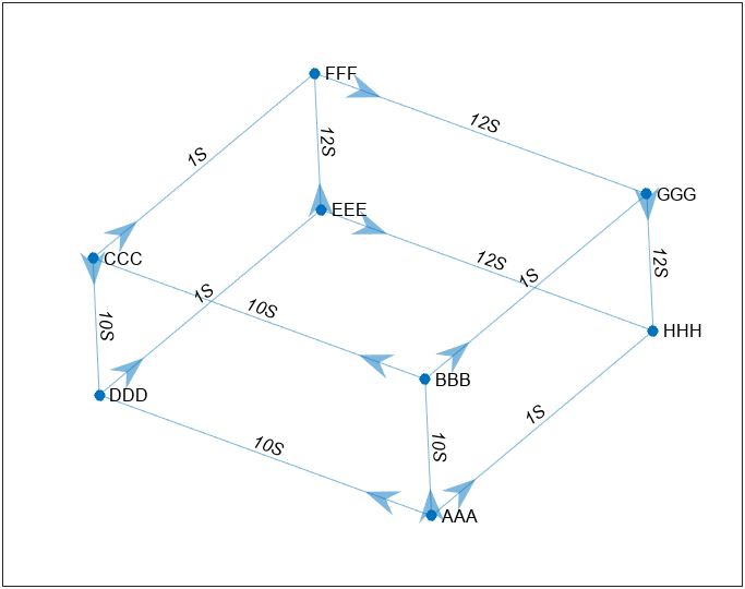
以下操作在如下例子的基础上进行: s=[1 1 1 2 2 3 3 4 5 5 6 7]; t=[2 4 8 3 7 4 6 5 6 8 7 8]; weights=[10 10 1 10 1 10 1 1 12 12 12 12]; names={'A' 'B' 'C' 'D' 'E' 'F' 'G' 'H'}; codeW={'10S','10S','1S','10S','1S','10S','1S','1S','12S','12S','12S','12S'}; codeN={'AAA' 'BBB' 'CCC' 'DDD' 'EEE' 'FFF' 'GGG' 'HHH'}; G=digraph(s,t,weights,names); h=plot(G,'EdgeLabel',codeW,'NodeLabel',codeN,'Layout','subspace');
线条粗细: h.LineWidth=weights;
线条颜色: h.EdgeColor=[0,0,0];
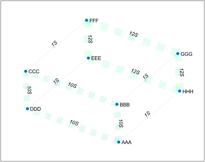
线条颜色映射: h.EdgeCData=weights; colormap(winter)
线条样式: h.LineStyle=':';
透明度: h.EdgeAlpha=.1;
节点大小: h.MarkerSize=(1:8).*3;
节点颜色: h.NodeColor='red';%[1,0,0]
节点颜色映射: h.NodeCData=1:8;
节点形状: h.Marker="^";
标签各个属性名就加个Node或者Edge即可: h.NodeFontName='Cambria'; h.NodeFontSize=15; h.NodeLabelColor=[0,0,.8];
箭头大小: h.ArrowSize=15;
箭头位置,范围0-1比例,0时代表在末尾,1时代表在头部 h.ArrowPosition=1;
老版本就可以像正常plot函数一样设置属性,属性设置可以写的比较随意,而且和普通plot含函数绘图非常类似,甚至这样都行: G=graph(bucky); plot(G,'-.dr','NodeLabel',{}) axis tight equal
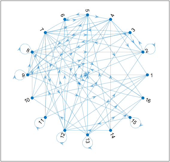
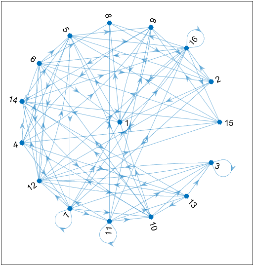
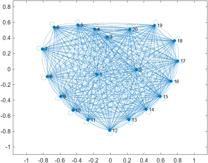
就是节点均匀分布在圆上: A=rand(16)>.7; G=digraph(A); plot(G,'Layout','circle') axis tight equal
把节点1放在中央: A=rand(16)>.7; G=digraph(A); plot(G,'Layout','circle','Center',1) axis tight equal
在相邻节点之间使用引力,在远距离节点之间使用斥力: s=[1 1 1 1 1 6 6 6 6 6 11 11 11]; t=[2 3 4 5 6 7 8 9 10 11 12 13 14]; G=graph(s,t); plot(G,'Layout','force');
增添权重影响,权重越大的边越长: s=[1 1 1 1 1 6 6 6 6 6 11 11 11]; t=[2 3 4 5 6 7 8 9 10 11 12 13 14]; weights=randi([1 20],1,13); G=graph(s,t,weights); plot(G,'Layout','force','WeightEffect','direct');
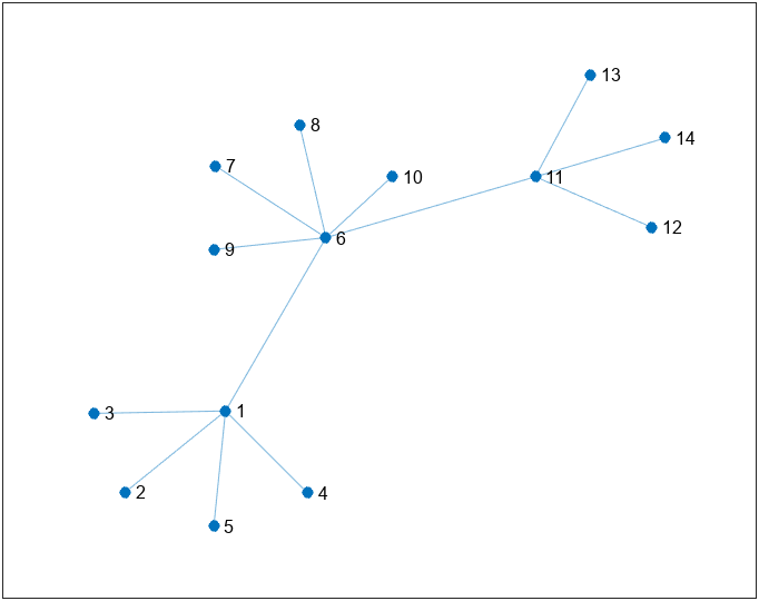
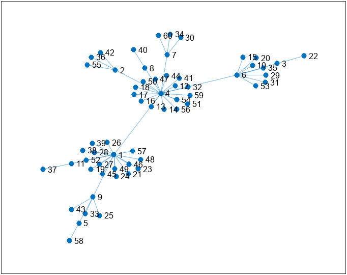
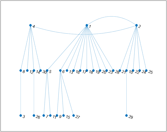
通过调整’Iterations’改变引力模拟迭代次数,以下举迭代10次和迭代1000次例子(迭代的初始X,Y坐标可通过’XStart’及’YStart’属性设置以保证每次实验结果相同,此处不再赘述): % 随便生成一组最小生成树 A=rand(60)>.7; G=graph(A,'upper'); T=minspantree(G); plot(T,'Layout','force','Iterations',10);
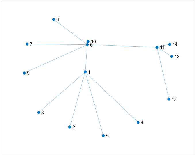
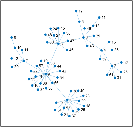
围绕原点: % 随便生成一组最小生成树 A=rand(60)>.7; G=graph(A,'upper'); T=minspantree(G); plot(T,'Layout','force','UseGravity',true); axis tight equal
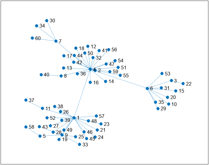
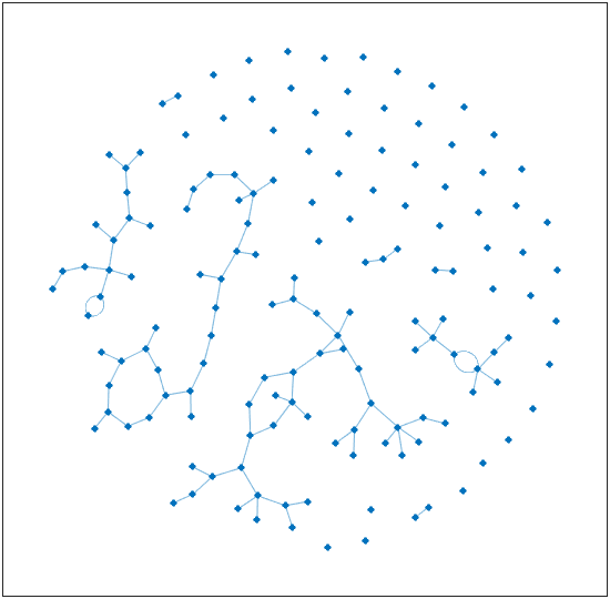
给个更直观的例子: s=[1 3 5 7 7 10:100]; t=[2 4 6 8 9 randi([10 100],1,91)]; G=graph(s,t,[],150); plot(G,'Layout','force','UseGravity',true); axis tight equal
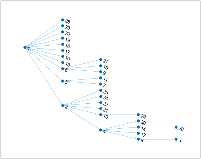
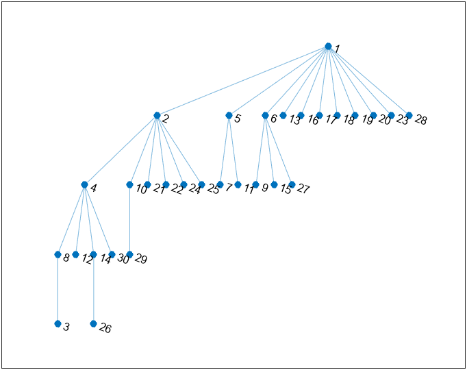
有层次的树状布局: % 随便生成一组最小生成树 A=rand(30)>.7; G=graph(A,'upper'); T=minspantree(G) plot(T,'Layout','layered')
通过设置’Direction’ 设置方向,可选为’down’ | ‘up’ | ‘left’ | ‘right’ plot(T,'Layout','layered','Direction','right')
'Sources’属性可用来设置哪些点在第一层,'Sinks’属性可用来设置哪些点在最后一层: plot(T,'Layout','layered','Sources',[1,2,4])
‘AssignLayers’属性可用来设置层分配方法,可选为’auto’ | ‘asap’ | ‘alap’ auto: 节点分配使用 ‘asap’ 或 ‘alap’,以两者中更紧凑者为准。asap: 在分配节点时,在满足该节点所有前趋节点都必须在其之前的层的约束条件下,将其分配到尽可能靠前的层。alap: 在分配节点时,在满足其所有后继节点都必须在其之后的层的约束条件下,将其分配到尽可能后的层。 plot(T,'Layout','layered','AssignLayers','asap')
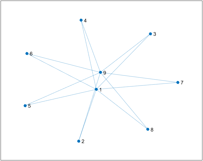
在高维嵌入式子空间中绘制图节点,然后将位置投影回二维。默认情况下,子空间维度是100或节点总数(以两者中较小者为准): s=[1 1 1 2 2 3 3 4 5 5 6 7]; t=[2 4 8 3 7 4 6 5 6 8 7 8]; G=graph(s,t); plot(G,'Layout','subspace');
通过’Dimension’设置高维空间维数。 XYZW=(abs(dec2bin(0:2^4-1))-48.5).*2; IPT=tril(XYZW*(XYZW')); [rows,cols]=find(IPT==2); G=graph(rows,cols); plot(G,'Layout','subspace');
与force布局可设置属性几乎完全一样不过是三维的: A=rand(30)>.7; G=graph(A,'upper'); T=minspantree(G); plot(T,'Layout','force3','UseGravity',true); axis tight equal
与subspace布局可设置属性几乎完全一样不过是三维的: XYZW=(abs(dec2bin(0:2^4-1))-48.5).*2; IPT=tril(XYZW*(XYZW')); [rows,cols]=find(IPT==2); G=graph(rows,cols); plot(G,'Layout','subspace3','Dimension',13);
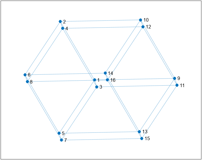
弄个心形: posXY=[-0.1598 -0.0682; 0.3117 -0.0060;-0.0389 0.4154;-0.1874 0.5155; -0.3877 0.5691;-0.6693 0.5397;-0.8092 0.2599;-0.7522 -0.0959; -0.5915 -0.3515;-0.4465 -0.5294;-0.2668 -0.6503;-0.0060 -0.7867; 0.2202 -0.6503; 0.4275 -0.5173; 0.5933 -0.3515; 0.7228 -0.1563; 0.8040 0.1045; 0.7642 0.3653; 0.5259 0.5622; 0.2323 0.5121]; A=ones(20)>0; [s,t]=find(A); G=graph(s,t); plot(G,'XData',posXY(:,1),'YData',posXY(:,2))
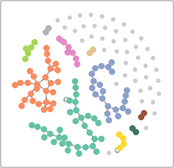
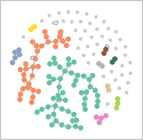
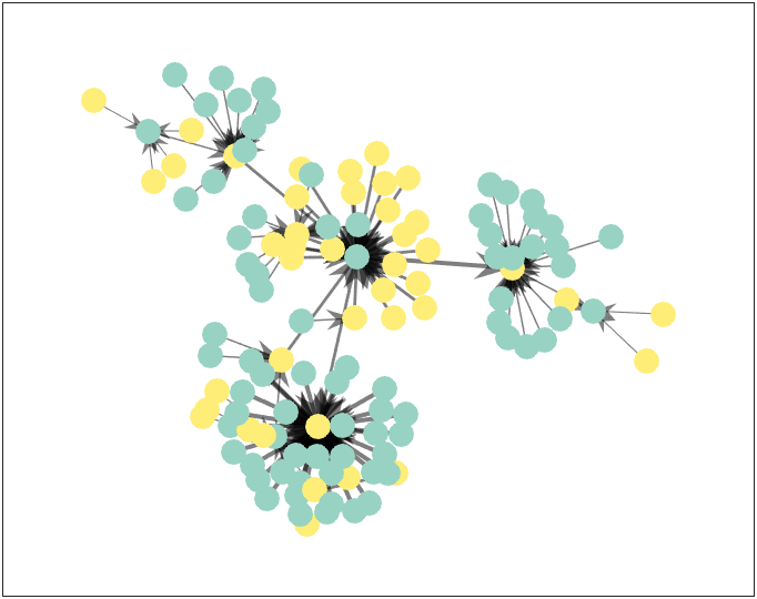
其实也算是给出一些好看的绘图模板叭,喜欢看的人多以后可以单独出几期绘图复刻啥的。 5.1 conncomp分类 s=[randi([1 50],1,40),randi([51 60],1,5),61:120]; t=[randi([1 50],1,40),randi([51 60],1,5),randi([61,120],1,60)]; G=graph(s,t,[],150); % 分割,并将孤立点归为一类 bins=conncomp(G); newBins=bins; tb=tabulate(bins); [~,ind]=sort(tb(:,2),'descend'); nV=tb(ind,1); nS=tb(ind,2); for i=1:length(ind) if nS(i)>1 newBins(bins==nV(i))=i; else newBins(bins==nV(i))=0; end end newBins=newBins+1; % 基础绘图 G=digraph(s,t,[],150); h=plot(G,'Layout','force','UseGravity',true); axis tight equal % 属性修饰 h.NodeCData=newBins; h.EdgeColor=[0,0,0]; h.EdgeAlpha=.3; h.LineWidth=2; h.MarkerSize=6+(newBins>1).*3; CM=[0.4000 0.7608 0.6471 0.9882 0.5529 0.3843 0.5529 0.6275 0.7961 0.9059 0.5412 0.7647 0.6510 0.8471 0.3294 1.0000 0.8510 0.1843 0.8980 0.7686 0.5804 0.7020 0.7020 0.7020]; CM=[CM;CM.*.6]; CM=[.8,.8,.8;CM]; colormap(CM(1:max(newBins),:))
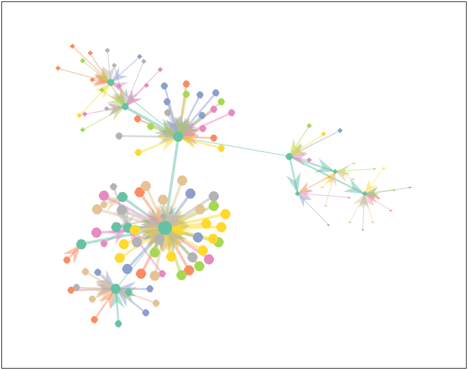
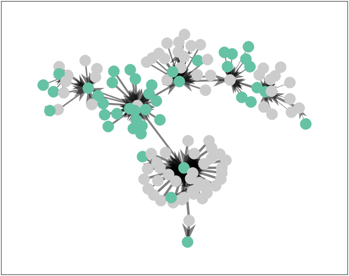
修改一下配色: n=120; A=rand(120)>.7; G=graph(A,'upper'); T=minspantree(G,'Root',1); L=zeros(1,n); for i=1:n L(i)=length(shortestpath(T,1,i)); end T=digraph(T.Edges.EndNodes(:,2),T.Edges.EndNodes(:,1)); % 基础绘图 h=plot(T,'Layout','force','Iterations',5); h.MarkerSize=10; h.LineWidth=(max(L(2:end))-L(2:end))./max(L(2:end)).*3+.1; h.ArrowSize=(max(L(2:end))-L(2:end))./max(L(2:end)).*10+10; h.ArrowPosition=1; % 设置配色 h.EdgeColor=[0,0,0]; h.NodeCData=mod(L,2)+1; CM=[.8,.8,.8 0.4000 0.7608 0.6471]; colormap(CM)
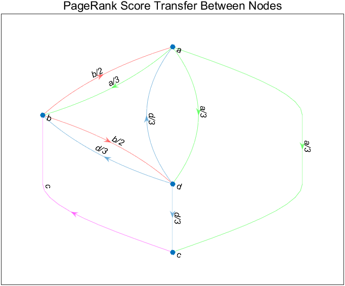
Watts-Strogatz 模型是一个包含小世界网络属性(例如集群和平均短路径长度)的随机图形。详细介绍请见: https://ww2.mathworks.cn/help/matlab/math/build-watts-strogatz-small-world-graph-model.html 创建 Watts-Strogatz 图形包含以下两个基本步骤: 创建一个环形网格,其中包含 N N N 个平均出入度为 2 K 2K 2K 的节点。每个节点都与任一侧的 K K K 个最近邻点相连。对于图中的每条边,重新连接概率为 β \beta β的目标节点。重新连接的边不能是重复或自环的。执行第一步操作之后,图形将是一个完美的环形网格。因此当 β = 0 \beta=0 β=0时,不会重新连接任何边,并且该模型会返回一个环形网格。而如果 β = 1 \beta=1 β=1,则所有边都将重新连接,并且环形网格会变成随机图形。 文件 WattsStrogatz.m 对无向图实现该图算法。根据上面的算法说明,输入参数为 N、K 和 beta。 % Copyright 2015 The MathWorks, Inc. function h = WattsStrogatz(N,K,beta) % H = WattsStrogatz(N,K,beta) returns a Watts-Strogatz model graph with N % nodes, N*K edges, mean node degree 2*K, and rewiring probability beta. % % beta = 0 is a ring lattice, and beta = 1 is a random graph. % Connect each node to its K next and previous neighbors. This constructs % indices for a ring lattice. s = repelem((1:N)',1,K); t = s + repmat(1:K,N,1); t = mod(t-1,N)+1; % Rewire the target node of each edge with probability beta for source=1:N switchEdge = rand(K, 1) 'b' 'c' 'd' 'd' 'a' 'b' 'c' 'a' 'b'}; G = digraph(s,t); labels = {'a/3' 'a/3' 'a/3' 'b/2' 'b/2' 'c' 'd/3' 'd/3' 'd/3'}; p = plot(G,'Layout','layered','EdgeLabel',labels); highlight(p,[1 1 1],[2 3 4],'EdgeColor','g') highlight(p,[2 2],[1 4],'EdgeColor','r') highlight(p,3,2,'EdgeColor','m') title('PageRank Score Transfer Between Nodes')
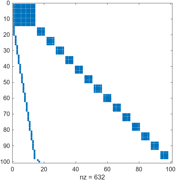
加载 mathworks100.mat 中的数据,并查看邻接矩阵 A。这些数据是使用自动网页趴chong程序在 2015 年生成的。网页趴chong程序从 https://www.mathworks.com 开始,然后是指向后续网页的链接,直到邻接矩阵包含 100 个唯一网页连接的相关信息。 load mathworks100.mat spy(A)
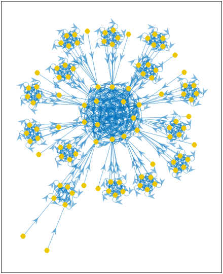
绘制网络图: load mathworks100.mat G=digraph(A,U); plot(G,'NodeLabel',{},'NodeColor',[0.93 0.78 0],'Layout','force'); axis tight equal
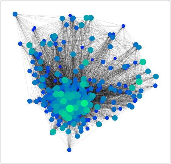
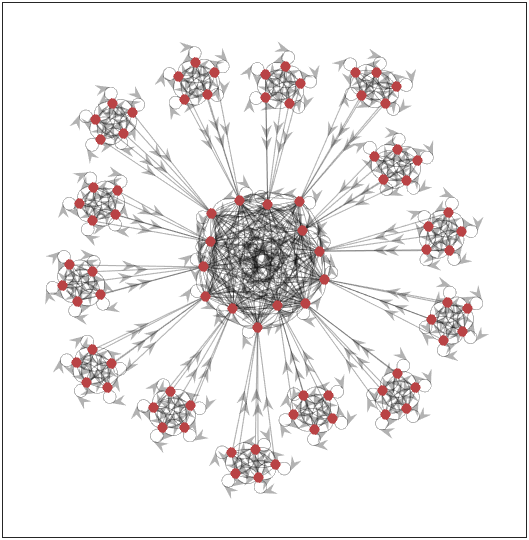
MATLAB自带centrality函数可以计算重要性: load mathworks100.mat G=digraph(A,U); pr = centrality(G,'pagerank','MaxIterations',200,'FollowProbability',0.85); G.Nodes.PageRank = pr; G.Nodes.InDegree = indegree(G); G.Nodes.OutDegree = outdegree(G); H=subgraph(G,find(G.Nodes.PageRank > 0.005)); h=plot(H,'NodeLabel',{},'NodeCData',H.Nodes.PageRank,'Layout','force'); colormap(parula(32)) colorbar axis tight equal
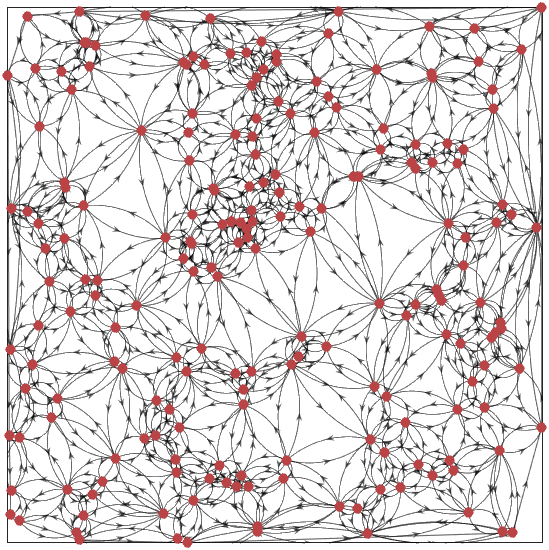
修改配色: h.EdgeColor=[0,0,0]; h.EdgeAlpha=.3; h.NodeColor=[185,67,69]./255; colorbar('off')
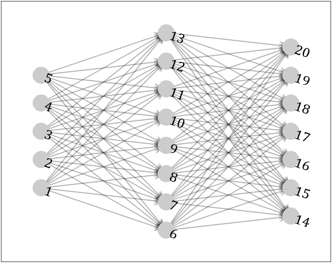
最多只能三层。三层往上建议自己写个函数。 layer=[5,8,7]; sumlayer=[0,cumsum(layer)]; S=[];T=[]; for i=1:length(layer)-1 [tS,tT]=meshgrid(1:layer(i),1:layer(i+1)); S=[S;tS(:)+sumlayer(i)]; T=[T;tT(:)+sumlayer(i+1)]; end G=digraph(S,T); h=plot(G,'Layout','layered','Sources',1:layer(1),'AssignLayers','asap',... 'Sinks',sumlayer(end-1)+1:sumlayer(end),'Direction','right'); h.ArrowPosition=1; h.LineWidth=1; h.EdgeColor=[0,0,0]; h.EdgeAlpha=.3; h.ArrowSize=12; h.MarkerSize=16; h.NodeColor=[.8,.8,.8]; h.NodeFontSize=14; h.NodeFontName='Cambria';
又是一篇大长文结束 攒着想写的文章总算又干掉一篇 网络图绘制技能树get 编写不易希望大家多多点赞!! 全部代码mlx文件请以下gitee仓库获取: https://gitee.com/slandarer/matlab-graph-plot |


【本文地址】
今日新闻 |
推荐新闻 |