Matlab作图中只显示特定区域内图像方法 |
您所在的位置:网站首页 › matlab删除图像的一部分 › Matlab作图中只显示特定区域内图像方法 |
Matlab作图中只显示特定区域内图像方法
|
Matlab作图中只显示特定区域内图像方法
参考链接中的例子, 已知一个二元函数 z=f(x,y)=3*(x.^2)+3*(y.^2)+3*x*y+1-3*x-3*y, 其定义域为 D={(x,y) | x>=0, y>=0, x+y 1; x(idx) = nan; y(idx) = nan; z = 3*(x.^2)+3*(y.^2)+3*x.*y+1-3*x-3*y; surf(x,y,z) % 或者 [x,y] = meshgrid(0:0.02:1); z = 3*(x.^2)+3*(y.^2)+3*x.*y+1-3*x-3*y; z(x+y>1) = nan; surf(x,y,z); axis tight
直接产生三角形定义域区域内的网格点。 n = 50; x = linspace(0,1,n+1); y = cumsum([zeros(size(x));repmat((1-x)/n,n,1)]); x = repmat(x,size(y,1),1); z = 3*(x.^2)+3*(y.^2)+3*x.*y+1-3*x-3*y; mesh(x,y,z); axis tight产生的原理是先让 x 方向上的点等间隔分布,再针对每个 x 在 y 方向上选取相同数量的等间隔分布的 y,最终的效果是网格点在 x 方向均匀分布,在 y 方向上分布的密度随着对应的 x 增大而逐渐增大(这是因为 y 的上限是一条斜线)。所以图形看起来会在接近 (0,1) 的一个角上变得非常密集 (体现在网格曲面颜色的改变上)。另一方面,由于这种方法是直接产生定义域内的点,在曲面边缘处的图形也是连续的。另外,此代码也可以修改成先产生等间隔分布的y,然后针对每个 y构建符合要求的 x,这样,就可以得到网格点在 y 方向均匀分布,在 x 方向非均匀分布。
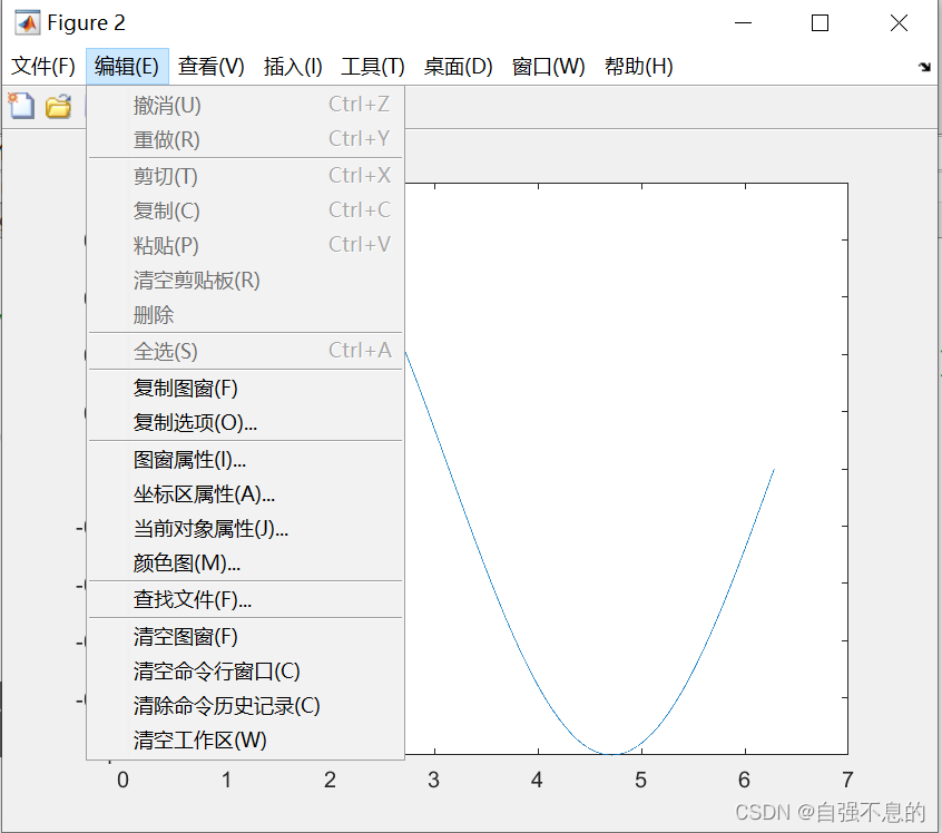
meshgrid 产生的是矩形网格,mesh、surf 函数是用矩形网格去呈现 3D 曲面 delaunay 产生的是三角形网格,对应的 trisurf、trimesh 函数是用三角形网格去呈现 3D 曲面 Matlab绘图去除坐标系及背景以及导出到visio在Matlab绘图时有时只想保留绘图的图形部分,不想要白色背景及坐标系,那么下面这段代码可以帮你解决这个问题 %去除上右边框刻度 box off %移除坐标轴边框 set(gca,'Visible','off'); set(gcf,'color','none'); set(gca,'color','none'); set(gcf,'InvertHardCopy','off');把上述代码放在画图的语句之后就可以获取到需要的透明图形了。然后可以复制到visio等画图软件。 导出到visio的方法尝试,plot画的线条图都可以 方法1:图形编辑器里点击:编辑–>复制图窗–>visio–>粘贴–>右键–>取消组合,针对波形还可以,针对三维图形波形质量不好,需要提升分辨率。 例子: figure; m=0:0.001:2*pi; plot(m,sin(m));
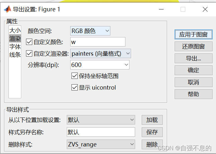
导出emf格式图片。 生成图片后,点击 “文件 -> 导出设置 ->渲染 -> 选中 painters(矢量格式)-> 应用于图窗”,同时建议把分辨率改为 600,关闭导出设置,点击 “文件 -> 另存为 -> 保存为 emf 格式”。因为 emf 格式可以直接在 visio 中打开,并进行二次编辑,visio 中 选中图片,点击 “组合 -> 取消组合”,删除自己不需要的。
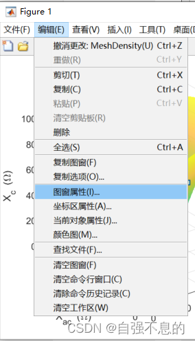
导出svg格式图片,通过测试,svg格式三维图导入到visio比emp格式效果好。 如果导出的图形不够清晰,可以对图窗属性中的MeshDensity适当加大(太大会导致卡住,甚至数组超过预设的最大数组大小),同时在 “文件 -> 导出设置 ->渲染 -> 选中 painters(矢量格式)-> 应用于图窗”,把分辨率改为 600。效果会明显改善。
对于Simulink的scope中的图,可用: 1、to workspace模块将scope的图导入工作空间; 2、直接利用示波器自带导出工具处理:设置示波器背景颜色为白色–>File–>Print to Figure 一些好用的函数介绍 slice 函数slice做出的图是在切片上用颜色表示v的值。有时,我们画切片图形也有助于我们理解一个4维图形。以 v= f(x,y,z) = xyz*exp(-(x2+y2+z^2)) 为例,假设我们希望看 v =f(x,y,z) 在 x =0, y = 1, z = 1 这些平面切片的图形,我们可以用以下代码: slice(X,Y,Z,V,xslice,yslice,zslice) 为三维体数据 V 绘制切片。指定 X、Y 和 Z 作为坐标数据。使用以下形式之一指定 xslice、yslice 和 zslice 作为切片位置: 要绘制一个或多个与特定轴正交的切片平面,请将切片参数指定为标量或向量。 要沿曲面绘制单个切片,请将所有切片参数指定为定义曲面的矩阵。 [x,y,z] = meshgrid(linspace(-2,2)); v = x.*y.*z.*exp(-(x.^2+y.^2+z.^2)); xslice = 0; yslice = 1; zslice = 1; slice(x,y,z,v,xslice,yslice,zslice) xlabel('x'); ylabel('y'); zlabel('z'); colormap hsv isosurface 等值面函数调用格式:fv = isosurface(X,Y,Z,V,isovalue) 作用:返回某个等值面(由isovalue指定)的表面(faces)和顶点(vertices)数据,存放在结构体fv中(fv由vertices、faces两个域构成)。如果是画隐函数 v = f(x,y,z) = 0 的三维图形,那么等值面的数值为isovalue = 0。 patch函数调用格式:patch(X,Y,C) 以平面坐标(X, Y)为顶点,构造平面多边形,C是RGB颜色向量 patch(X,Y,Z,C)以空间3-D坐标(X, Y,Z)为顶点,构造空间3D曲面,C是RGB颜色向量 patch(fv) 通过包含vertices、faces两个域的结构体fv来构造3D曲面,fv可以直接由等值面函数isosurface得到 例如:patch(isosurface(X,Y,Z,V,0)) isonormals等值面法线函数调用格式:isonormals(X,Y,Z,V,p) 实现功能:计算等值面V的顶点法线,将patch曲面p的法线设置为计算得到的法线(p是patch返回得到的句柄)。如果不设置法线的话,得到曲面在过渡地带看起来可能不是很光滑 ezimplot3 函数获取:http://www.mathworks.com/matlabcentral/fileexchange/23623-ezimplot3-implicit-3d-functions-plotter 声明:这个是上述网站链接的内容,因为为办法免费上传,只能贴代码了。 % Copyright (c) 2009, Gustavo Morales % All rights reserved. function h = ezimplot3(varargin) % EZIMPLOT3 Easy to use 3D implicit plotter. % EZIMPLOT3(FUN) plots the function FUN(X,Y,Z) = 0 (vectorized or not) % over the default domain: % -2*PI < X < 2*PI, -2*PI < Y < 2*PI, -2*PI < Z < 2*PI. % FUN can be a string, an anonymous function handle, a .M-file handle, an % inline function or a symbolic function (see examples below) % % EZIMPLOT3(FUN,DOMAIN)plots FUN over the specified DOMAIN instead of the % default domain. DOMAIN can be vector [XMIN,XMAX,YMIN,YMAX,ZMIN,ZMAX] or % vector [A,B] (to plot over A < X < B, A < Y < B, A < Z < B). % % EZIMPLOT3(..,N) plots FUN using an N-by-N grid. The default value for % N is 60. % EZIMPLOT3(..,'color') plots FUN with color 'color'. The default value % for 'color' is 'red'. 'color' must be a valid Matlab color identifier. % % EZIMPLOT3(axes_handle,..) plots into the axes with handle axes_handle % instead of into current axes (gca). % % H = EZIMPLOT3(...) returns the handle to the patch object this function % creates. % % Example: % Plot x^3+exp(y)-cosh(z)=4, between -5 and 5 for x,y and z % % via a string: % f = 'x^3+exp(y)-cosh(z)-4' % ezimplot3(f,[-5 5]) % % via a anonymous function handle: % f = @(x,y,z) x^3+exp(y)-cosh(z)-4 % ezimplot3(f,[-5 5]) % % via a function .m file: %------------------------------% % function out = myfun(x,y,z) % out = x^3+exp(y)-cosh(z)-4; %------------------------------% % ezimplot3(@myfun,[-5 5]) or ezimplot('myfun',[-5 5]) % % via a inline function: % f = inline('x^3+exp(y)-cosh(z)-4') % ezimplot3(f,[-5 5]) % % via a symbolic expression: % syms x y z % f = x^3+exp(y)-cosh(z)-4 % ezimplot3(f,[-5 5]) % % Note: this function do not use the "ezgraph3" standard, like ezsurf, % ezmesh, etc, does. Because of this, ezimplot3 only tries to imitate that % interface. A future work must be to modify "ezgraph3" to include a % routine for implicit surfaces based on this file % % Inspired by works of: Artur Jutan UWO 02-02-98 [email protected] % Made by: Gustavo Morales UC 04-12-09 [email protected] % %%% Checking & Parsing input arguments: if ishandle(varargin{1}) cax = varargin{1}; % User selected axes handle for graphics axes(cax); args{:} = varargin{2:end}; %ensuring args be a cell array else args = varargin; end [fun domain n color] = argcheck(args{:}); %%% Generating the volumetric domain data: xm = linspace(domain(1),domain(2),n); ym = linspace(domain(3),domain(4),n); zm = linspace(domain(5),domain(6),n); [x,y,z] = meshgrid(xm,ym,zm); %%% Formatting "fun" [f_handle f_text] = fix_fun(fun); % f_handle is the anonymous f-handle for "fun" % f_text is "fun" ready to be a title %%% Evaluating "f_handle" in domain: try fvalues = f_handle(x,y,z); % fvalues: volume data catch ME error('Ezimplot3:Functions', 'FUN must have no more than 3 arguments'); end %%% Making the 3D graph of the 0-level surface of the 4D function "fun": h = patch(isosurface(x,y,z,fvalues,0)); % "patch" handles the structure... % sent by "isosurface" isonormals(x,y,z,fvalues,h)% Recalculating the isosurface normals based... % on the volume data set(h,'FaceColor',color,'EdgeColor','none'); %%% Aditional graphic details: xlabel('x');ylabel('y');zlabel('z');% naming the axis alpha(0.7) % adjusting for some transparency grid on; view([1,1,1]); axis equal; camlight; lighting gouraud %%% Showing title: title([f_text,' = 0']); % %--------------------------------------------Sub-functions HERE--- function [f dom n color] = argcheck(varargin) %ARGCHECK(arg) parses "args" to the variables "f"(function),"dom"(domain) %,"n"(grid size) and "c"(color)and TRIES to check its validity switch nargin case 0 error('Ezimplot3:Arguments',... 'At least "fun" argument must be given'); case 1 f = varargin{1}; dom = [-2*pi, 2*pi]; % default domain: -2*pi < xi < 2*pi n = 60; % default grid size color = 'red'; % default graph color case 2 f = varargin{1}; if isa(varargin{2},'double') && length(varargin{2})>1 dom = varargin{2}; n = 60; color = 'red'; elseif isa(varargin{2},'double') && length(varargin{2})==1 n = varargin{2}; dom = [-2*pi, 2*pi]; color = 'red'; elseif isa(varargin{2},'char') dom = [-2*pi, 2*pi]; n = 60; color = varargin{2}; end case 3 % If more than 2 arguments are given, it's f = varargin{1}; % assumed they are in the correct order dom = varargin{2}; n = varargin{3}; color = 'red'; % default color case 4 % If more than 2 arguments are given, it's f = varargin{1}; % assumed they are in the correct order dom = varargin{2}; n = varargin{3}; color = varargin{4}; otherwise warning('Ezimplot3:Arguments', ... 'Attempt will be made only with the 4 first arguments'); f = varargin{1}; dom = varargin{2}; n = varargin{3}; color = varargin{4}; end if length(dom) == 2 dom = repmat(dom,1,3); %domain repeated in all variables elseif length(dom) ~= 6 error('Ezimplot3:Arguments',... 'Input argument "domain" must be a row vector of size 2 or size 6'); end % %-------------------------------------------- function [f_hand f_text] = fix_fun(fun) % FIX_FUN(fun) Converts "fun" into an anonymous function of 3 variables (x,y,z) % with handle "f_hand" and a string "f_text" to use it as title types = {'char','sym','function_handle','inline'}; % cell array of 'types' type = ''; %Identifing FUN object class for i=1:size(types,2) if isa(fun,types{i}) type = types{i}; break; end end switch type case 'char' % Formatting FUN if it is char type. There's 2 possibilities: % A string with the name of the .m file if exist([fun,'.m'],'file') syms x y z; if nargin(str2func(fun)) == 3 f_sym = eval([fun,'(x,y,z)']); % evaluating FUN at the sym point (x,y,z) else error('Ezimplot3:Arguments',... '%s must be a function of 3 arguments or unknown function',fun); end f_text = strrep(char(f_sym),' ',''); % converting to char and eliminating spaces f_hand = eval(['@(x,y,z)',vectorize(f_text),';']); % converting string to anonymous f_handle else % A string with the function's expression f_hand = eval(['@(x,y,z)',vectorize(fun),';']); % converting string to anonymous f_handle f_text = strrep(fun,'.',''); f_text = strrep(f_text,' ',''); % removing vectorization & spaces end case 'sym' % Formatting FUN if it is a symbolic object f_hand = eval(['@(x,y,z)',vectorize(fun),';']); % converting string to anonymous f_handle f_text = strrep(char(fun),' ',''); % removing spaces case {'function_handle', 'inline'} % Formatting FUN if it is a function_handle or an inline object syms x y z; if nargin(fun) == 3 && numel(symvar(char(fun))) == 3 % Determining if # variables == 3 f_sym = fun(x,y,z); % evaluating FUN at the sym point (x,y,z) else error('Ezimplot3:Arguments',... '%s must be function of 3 arguments or unknown function',char(fun)); end f_text = strrep(char(f_sym),' ',''); % converting into string to removing spaces f_hand = eval(['@(x,y,z)',vectorize(f_text),';']); % converting string to anonymous f_handle otherwise error('First argument "fun" must be of type character, simbolic, function handle or inline'); endezimplot3使用方法:复制上述内容,保存为 ezimplot3.m 添加到matlab当前搜索路径后就可以使用了。推荐放到如下路径: C:\Program Files\MATLAB\R2013a\toolbox\matlab\datafun ezimplot3一共有三种参数调用方式: ezimplot3(f) 画函数f(X,Y,Z)= 0 在-2pi< X < 2 pi, -2* pi < Y < 2* pi, -2* pi < Z < 2* pi上的图形 ezimplot3(f, [A,B])画函数f(X,Y,Z)= 0 在A< X < B, A < Y < B, A < Z < B上的图形 ezimplot3(f, [XMIN,XMAX,YMIN,YMAX,ZMIN,ZMAX])画函数f(X,Y,Z)= 0 在XMIN< X < XMAX, YMIN < Y < YMAX, ZMIN < Z < ZMAX上的图形 隐函数谈论,论坛内容链接: https://www.ilovematlab.cn/thread-264471-1-1.html?_dsign=30357616 三维隐函数作图并且导出图像数据: https://www.ilovematlab.cn/thread-541481-1-1.html?s_tid=RelatedContent&_dsign=406099c7 4D-plot: https://www.ilovematlab.cn/thread-265517-1-1.html?_dsign=3726cac5 参考文献:以上内容都是对链接的内容整理总结。详细请参考如下链接 参考链接: 链接: link 链接: link 链接: link 链接: link 链接: link 参考项目: 链接: link 链接: link 其他工具: 链接: link https://ww2.mathworks.cn/matlabcentral/fileexchange/32506-marching-cubes |
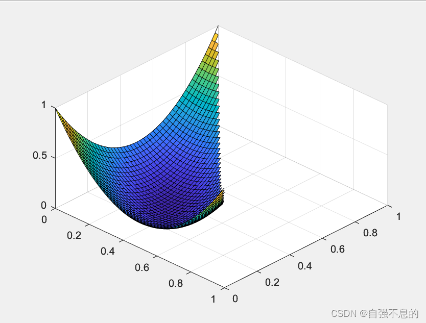 核心思想: 先产生矩形区域内均匀分布的网格数据,然后剔除不符合要求(即落在定义域以外)的网格点。这种办法能保证产生的网格点在 x 方向、y 方向都是均匀分布(体现在网格曲面上一般不会出现颜色的突变)。但是因为这种方法是直接将不符合要求的数据置为NAN,在图形的斜线边缘处(即 x+y=1的地方)会出现图形过度是不连续的,下面对其改进:
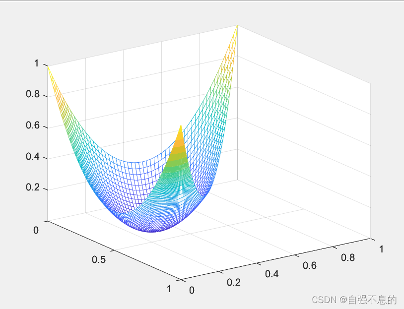 函数介绍:
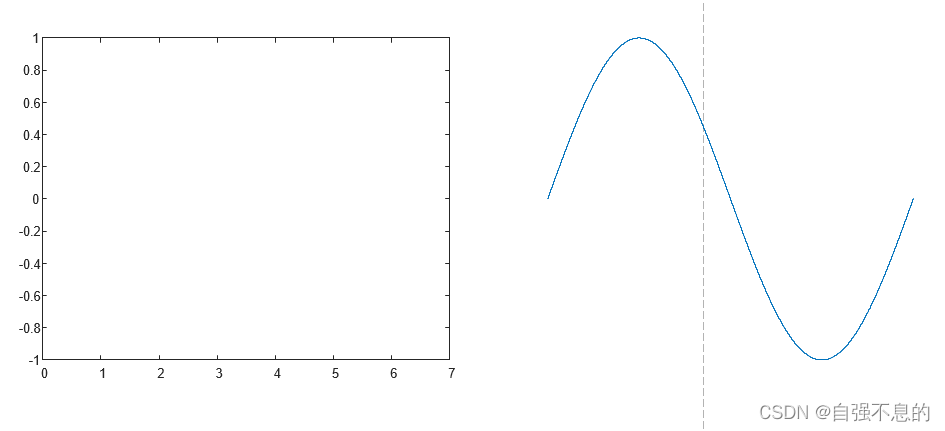
函数介绍: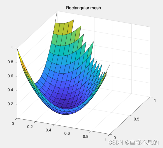 上图边界处不连续是因为该方法野蛮地将定义域外置nan。如果想提高这种方法边界处的连续性,需要让网格点变得更密(即meshgrid里的步长变得更小)
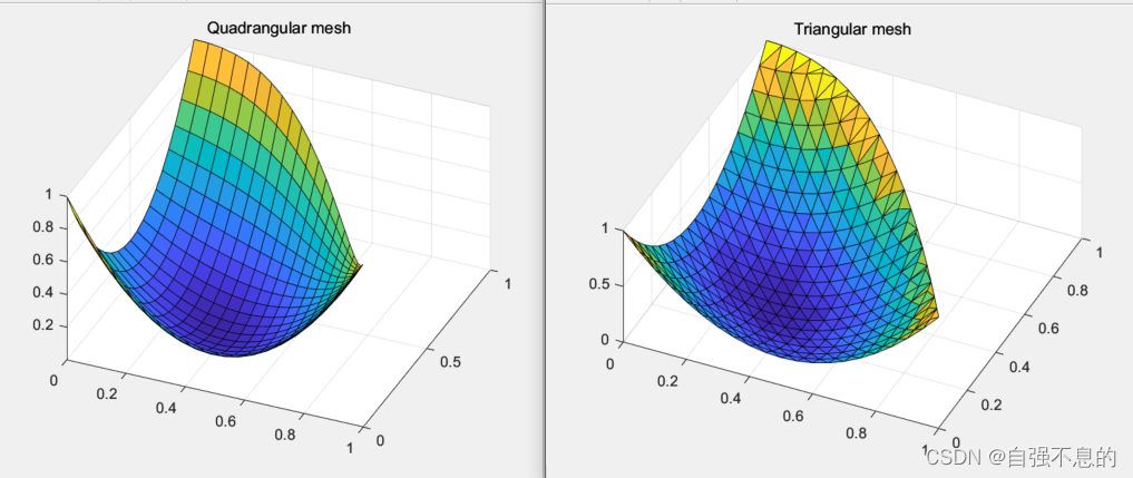
 预设项记得改一下
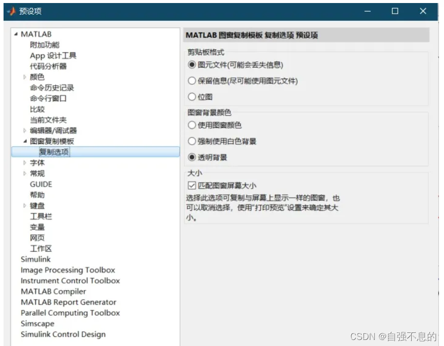
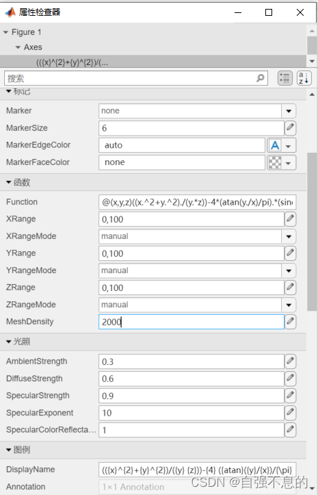 MeshDensity 太大
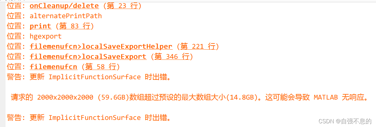
【本文地址】
今日新闻 |
推荐新闻 |