|
基于生存分析模型的用户流失预测 小O:有没有什么很好的办法在预测用户流失的同时,提供一些建议帮助我们运营呢? 小H:这简单,如果我可以告诉你什么样的人群容易流失、什么时间点容易流失、用户的可能存活多节可以吗? 小O:这太可以了~ 生存模型就能很好的地解决上面的问题,生存分析(Survival analysis)是指根据历史数据对人的生存时间进行分析和推断,研究生存情况与众多影响因素间的关系。本文参考自python数据分析案例-利用生存分析Kaplan-Meier法与COX比例风险回归模型进行客户流失分析与剩余价值预测。 数据探索导入相关库# pip install -i https://pypi.doubanio.com/simple/ lifelines # 采用镜像安装
import pandas as pd
import numpy as np
import matplotlib.pyplot as plt
import seaborn as sns
from lifelines import NelsonAalenFitter, CoxPHFitter, KaplanMeierFitter
from lifelines.statistics import logrank_test, multivariate_logrank_test
from sklearn.model_selection import train_test_split, GridSearchCV
from lifelines.utils.sklearn_adapter import sklearn_adapter
from sklearn import metrics
import time
import math
import toad
import itertools
from lifelines.plotting import add_at_risk_counts
from lifelines.statistics import pairwise_logrank_test
from sklearn import preprocessing
from lifelines.calibration import survival_probability_calibration
from sklearn.metrics import brier_score_loss
from lifelines.utils import median_survival_times, qth_survival_times
plt.rcParams['font.sans-serif'] = ['SimHei']
plt.rcParams['axes.unicode_minus'] = False
import warnings
warnings.filterwarnings("ignore")
数据准备 以下数据如果有需要的同学可关注公众号HsuHeinrich,回复【数据挖掘-生存分析】自动获取~ # 读取数据
raw_data = pd.read_csv('Customer-Churn.csv')
raw_data.head()
 image-20230206152049606数据预处理df = raw_data.copy()
# 删除tenure=0(This model does not allow for non-positive durations)
df = df[df['tenure']>0]
# 转换成连续型变量
df['TotalCharges'] = pd.to_numeric(df.TotalCharges, errors='coerce')
# 填充缺失值
df['TotalCharges'].fillna(0, inplace=True)
# 转换成类别变量
df['SeniorCitizen'] = df['SeniorCitizen'].astype("str")
# 将是否流失转换为01分布
df['Churn'] = df['Churn'].map({'No':0,'Yes':1})
生存分析探索查看整体生存曲线fig, ax = plt.subplots(nrows=2, ncols=1, figsize=(12,10))
# 整体生存曲线
kmf = KaplanMeierFitter()
kmf.fit(df.tenure, # 代表生存时长
event_observed=df.Churn # 代表事件的终点
)
kmf.plot_survival_function(ax=ax[0], label='all')
ax[0].grid()
# 整体生存变化率
naf = NelsonAalenFitter()
naf.fit(df.tenure, event_observed=df.Churn)
naf.plot_hazard(ax=ax[1], bandwidth=20, label='all')
ax[1].grid()
plt.show() image-20230206152049606数据预处理df = raw_data.copy()
# 删除tenure=0(This model does not allow for non-positive durations)
df = df[df['tenure']>0]
# 转换成连续型变量
df['TotalCharges'] = pd.to_numeric(df.TotalCharges, errors='coerce')
# 填充缺失值
df['TotalCharges'].fillna(0, inplace=True)
# 转换成类别变量
df['SeniorCitizen'] = df['SeniorCitizen'].astype("str")
# 将是否流失转换为01分布
df['Churn'] = df['Churn'].map({'No':0,'Yes':1})
生存分析探索查看整体生存曲线fig, ax = plt.subplots(nrows=2, ncols=1, figsize=(12,10))
# 整体生存曲线
kmf = KaplanMeierFitter()
kmf.fit(df.tenure, # 代表生存时长
event_observed=df.Churn # 代表事件的终点
)
kmf.plot_survival_function(ax=ax[0], label='all')
ax[0].grid()
# 整体生存变化率
naf = NelsonAalenFitter()
naf.fit(df.tenure, event_observed=df.Churn)
naf.plot_hazard(ax=ax[1], bandwidth=20, label='all')
ax[1].grid()
plt.show()
 output_8_0截至观察期(最大70个月),整体还有60%的用户未流失。不存在半衰期,即当用户流失达到50%的时间节点0-10个月用户流失加快,50-60个月的用户流失速率也有所提升# 缩短时间查看前20个月
t = np.linspace(0, 20, 21)
fig, ax = plt.subplots(nrows=2, ncols=1, figsize=(12,10))
# 整体生存曲线
kmf = KaplanMeierFitter()
kmf.fit(df.tenure, # 代表生存时长
event_observed=df.Churn, # 代表事件的终点
timeline=t
)
kmf.plot_survival_function(ax=ax[0], label='all')
# 整体生存变化率
naf = NelsonAalenFitter()
naf.fit(df.tenure, event_observed=df.Churn, timeline=t)
naf.plot_hazard(ax=ax[1], bandwidth=20, label='all')
plt.show() output_8_0截至观察期(最大70个月),整体还有60%的用户未流失。不存在半衰期,即当用户流失达到50%的时间节点0-10个月用户流失加快,50-60个月的用户流失速率也有所提升# 缩短时间查看前20个月
t = np.linspace(0, 20, 21)
fig, ax = plt.subplots(nrows=2, ncols=1, figsize=(12,10))
# 整体生存曲线
kmf = KaplanMeierFitter()
kmf.fit(df.tenure, # 代表生存时长
event_observed=df.Churn, # 代表事件的终点
timeline=t
)
kmf.plot_survival_function(ax=ax[0], label='all')
# 整体生存变化率
naf = NelsonAalenFitter()
naf.fit(df.tenure, event_observed=df.Churn, timeline=t)
naf.plot_hazard(ax=ax[1], bandwidth=20, label='all')
plt.show()
 output_10_0第一个月是用户流失重灾时间前10个月中,前5个月流失速率加快查看单变量生存曲线差异# 连续变量分箱
combiner = toad.transform.Combiner()
combiner.fit(df[['MonthlyCharges','TotalCharges']], df['Churn'], method='chi', # 卡方分箱
min_samples=0.05)
df_t = combiner.transform(df)
# 筛选变量
obj_list = df_t.select_dtypes(include="object").columns[1:].to_list()
obj_list += ['MonthlyCharges','TotalCharges']
# 计算行列数
num_plots = len(obj_list)
num_cols = math.ceil(np.sqrt(num_plots))
num_rows = math.ceil(num_plots/num_cols)
cr = [d for d in itertools.product(range(num_rows),range(num_cols))]
# 绘制生存曲线
fig, ax = plt.subplots(nrows=num_rows, ncols=num_cols, figsize=(48,36))
for ind,feature in enumerate(obj_list):
for i in df_t[feature].unique():
# KaplanMeier检验
kmf=KaplanMeierFitter()
df_tmp = df_t.loc[df_t[feature] == i]
kmf.fit(df_tmp.tenure, # 代表生存时长
event_observed=df_tmp.Churn, # 代表事件的终点
label=i)
# 绘制生存曲线
kmf.plot_survival_function(ci_show=False,
ax = ax[cr[ind][0]][cr[ind][1]])
# 对数秩检验,得到p值
p_value = multivariate_logrank_test(event_durations = df_t.tenure, # 代表生存时长
groups=df_t[feature], # 代表检验的组别
event_observed=df_t.Churn # 代表事件的终点
).p_value
p_value_text = ['p-value < 0.001' if p_value output_13_0验证多分类单变量生存曲线差异# 查看多分类变量的组间差异:以PaymentMethod为例
fig, ax = plt.subplots(figsize=(10,6))
feature = 'PaymentMethod'
for i in df_t[feature].unique():
# KaplanMeier检验
kmf=KaplanMeierFitter()
df_tmp = df_t.loc[df_t[feature] == i]
kmf.fit(df_tmp.tenure, # 代表生存时长
event_observed=df_tmp.Churn, # 代表事件的终点
label=i)
# 绘制生存曲线
kmf.plot_survival_function(ci_show=False,
ax = ax)
# 对数秩检验,得到p值
p_value = multivariate_logrank_test(event_durations = df_t.tenure, # 代表生存时长
groups=df_t[feature], # 代表检验的组别
event_observed=df_t.Churn # 代表事件的终点
).p_value
p_value_text = ['p-value < 0.001' if p_value image-20221221185003629生存曲线表明PaymentMethod存在组间显著差异检验表明除了Bank transfer (automatic)与Credit card (automatic)不存在显著差异,其余组间均显著差异交互变量的生存曲线# 以性别gender为例,查看与其他变量交互后,gender的流失情况是否存在显著差异
for feature in obj_list:
for i in df_t[feature].unique():
df_tmp = df_t.loc[df_t[feature] == i]
p_value = multivariate_logrank_test(event_durations = df_tmp.tenure,
groups=df_tmp.gender,
event_observed=df_tmp.Churn
).p_value
if p_value output_20_0 在Credit card (automatic)客户中,Female更容易流失 特征工程# 特征工程
df_model = pd.get_dummies(df.iloc[:,1:], drop_first=True) # 剔除客户ID,并对类别变量进行哑变量处理(剔除首列防止虚拟变量陷阱)
# 拆分训练集
train, test = train_test_split(df_model, test_size=0.2)
数据建模模型拟合# 模型拟合
cph = CoxPHFitter(penalizer = 0.01)
cph.fit(train, duration_col='tenure', event_col='Churn')
cph.print_summary(decimals=1)
modellifelines.CoxPHFitterduration col'tenure'event col'Churn'penalizer0.01l1 ratio0baseline estimationbreslownumber of observations5625number of events observed1500partial log-likelihood-10138.3time fit was run2022-09-16 15:52:24 UTC output_10_0第一个月是用户流失重灾时间前10个月中,前5个月流失速率加快查看单变量生存曲线差异# 连续变量分箱
combiner = toad.transform.Combiner()
combiner.fit(df[['MonthlyCharges','TotalCharges']], df['Churn'], method='chi', # 卡方分箱
min_samples=0.05)
df_t = combiner.transform(df)
# 筛选变量
obj_list = df_t.select_dtypes(include="object").columns[1:].to_list()
obj_list += ['MonthlyCharges','TotalCharges']
# 计算行列数
num_plots = len(obj_list)
num_cols = math.ceil(np.sqrt(num_plots))
num_rows = math.ceil(num_plots/num_cols)
cr = [d for d in itertools.product(range(num_rows),range(num_cols))]
# 绘制生存曲线
fig, ax = plt.subplots(nrows=num_rows, ncols=num_cols, figsize=(48,36))
for ind,feature in enumerate(obj_list):
for i in df_t[feature].unique():
# KaplanMeier检验
kmf=KaplanMeierFitter()
df_tmp = df_t.loc[df_t[feature] == i]
kmf.fit(df_tmp.tenure, # 代表生存时长
event_observed=df_tmp.Churn, # 代表事件的终点
label=i)
# 绘制生存曲线
kmf.plot_survival_function(ci_show=False,
ax = ax[cr[ind][0]][cr[ind][1]])
# 对数秩检验,得到p值
p_value = multivariate_logrank_test(event_durations = df_t.tenure, # 代表生存时长
groups=df_t[feature], # 代表检验的组别
event_observed=df_t.Churn # 代表事件的终点
).p_value
p_value_text = ['p-value < 0.001' if p_value output_13_0验证多分类单变量生存曲线差异# 查看多分类变量的组间差异:以PaymentMethod为例
fig, ax = plt.subplots(figsize=(10,6))
feature = 'PaymentMethod'
for i in df_t[feature].unique():
# KaplanMeier检验
kmf=KaplanMeierFitter()
df_tmp = df_t.loc[df_t[feature] == i]
kmf.fit(df_tmp.tenure, # 代表生存时长
event_observed=df_tmp.Churn, # 代表事件的终点
label=i)
# 绘制生存曲线
kmf.plot_survival_function(ci_show=False,
ax = ax)
# 对数秩检验,得到p值
p_value = multivariate_logrank_test(event_durations = df_t.tenure, # 代表生存时长
groups=df_t[feature], # 代表检验的组别
event_observed=df_t.Churn # 代表事件的终点
).p_value
p_value_text = ['p-value < 0.001' if p_value image-20221221185003629生存曲线表明PaymentMethod存在组间显著差异检验表明除了Bank transfer (automatic)与Credit card (automatic)不存在显著差异,其余组间均显著差异交互变量的生存曲线# 以性别gender为例,查看与其他变量交互后,gender的流失情况是否存在显著差异
for feature in obj_list:
for i in df_t[feature].unique():
df_tmp = df_t.loc[df_t[feature] == i]
p_value = multivariate_logrank_test(event_durations = df_tmp.tenure,
groups=df_tmp.gender,
event_observed=df_tmp.Churn
).p_value
if p_value output_20_0 在Credit card (automatic)客户中,Female更容易流失 特征工程# 特征工程
df_model = pd.get_dummies(df.iloc[:,1:], drop_first=True) # 剔除客户ID,并对类别变量进行哑变量处理(剔除首列防止虚拟变量陷阱)
# 拆分训练集
train, test = train_test_split(df_model, test_size=0.2)
数据建模模型拟合# 模型拟合
cph = CoxPHFitter(penalizer = 0.01)
cph.fit(train, duration_col='tenure', event_col='Churn')
cph.print_summary(decimals=1)
modellifelines.CoxPHFitterduration col'tenure'event col'Churn'penalizer0.01l1 ratio0baseline estimationbreslownumber of observations5625number of events observed1500partial log-likelihood-10138.3time fit was run2022-09-16 15:52:24 UTC image-20221221185924375Concordance=0.9,模型拟合不错。Concordance Index是AUC的推广,值越接近1效果越好系数为正则表示该变量促进流失,系数为负表示该变量防止流失显著影响的为p0.05].index)
train_s = train.drop(drop_col, axis=1)
test_s = test.drop(drop_col, axis=1)
# 重新拟合
cph = CoxPHFitter(penalizer = 0.01)
cph.fit(train_s, duration_col='tenure', event_col='Churn')
cph.print_summary(decimals=1) image-20221221185924375Concordance=0.9,模型拟合不错。Concordance Index是AUC的推广,值越接近1效果越好系数为正则表示该变量促进流失,系数为负表示该变量防止流失显著影响的为p0.05].index)
train_s = train.drop(drop_col, axis=1)
test_s = test.drop(drop_col, axis=1)
# 重新拟合
cph = CoxPHFitter(penalizer = 0.01)
cph.fit(train_s, duration_col='tenure', event_col='Churn')
cph.print_summary(decimals=1)
 image-20221221190131160特征重要性# 特征重要性
fig,ax = plt.subplots(figsize=(12,9))
cph.plot(ax=ax)
plt.show() image-20221221190131160特征重要性# 特征重要性
fig,ax = plt.subplots(figsize=(12,9))
cph.plot(ax=ax)
plt.show()
 output_27_0加速流失的变量有:InternetService_Fiber optic、PaymentMethod_Mailed check等防止流失的变量有:Contract_Two year、Contract_One year等风险观察# 累积风险曲线
fig,ax = plt.subplots(nrows=2, ncols=1, figsize=(10,12))
cph.baseline_cumulative_hazard_.plot(ax=ax[0])
# 各时间节点的风险曲线
cph.baseline_hazard_.plot(ax=ax[1])
plt.show() output_27_0加速流失的变量有:InternetService_Fiber optic、PaymentMethod_Mailed check等防止流失的变量有:Contract_Two year、Contract_One year等风险观察# 累积风险曲线
fig,ax = plt.subplots(nrows=2, ncols=1, figsize=(10,12))
cph.baseline_cumulative_hazard_.plot(ax=ax[0])
# 各时间节点的风险曲线
cph.baseline_hazard_.plot(ax=ax[1])
plt.show()
 output_29_0 在60个月以后流失风险明显提高模型评估# 模型校准性
fig,ax = plt.subplots(figsize=(12,9))
survival_probability_calibration(cph, test_s, t0=50, ax=ax)
ax.grid()
ICI = 0.05854302858419381
E50 = 0.021989969295193035 output_29_0 在60个月以后流失风险明显提高模型评估# 模型校准性
fig,ax = plt.subplots(figsize=(12,9))
survival_probability_calibration(cph, test_s, t0=50, ax=ax)
ax.grid()
ICI = 0.05854302858419381
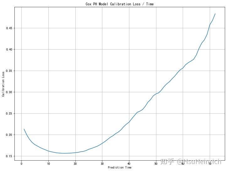
E50 = 0.021989969295193035 output_32_1x轴为预测的流失概率,y轴为观测的流失概率以50个月为例,模型与基准值(对角线)偏离较大,且一直高估了用户的流失情况建议样本均衡处理,剔除具有相关性的特征等# 使用brier score观测校准距离:Brier分数对于一组预测值越低,预测校准越好
loss_dict = {}
for i in range(1,73):
score = brier_score_loss(
test_s.Churn,
1 - np.array(cph.predict_survival_function(test_s).loc[i]),
pos_label=1 )
loss_dict[i] = [score]
loss_df = pd.DataFrame(loss_dict).T
fig, ax = plt.subplots(figsize=(12,9))
ax.plot(loss_df.index, loss_df)
ax.set(xlabel='Prediction Time', ylabel='Calibration Loss', title='Cox PH Model Calibration Loss / Time')
ax.grid() output_32_1x轴为预测的流失概率,y轴为观测的流失概率以50个月为例,模型与基准值(对角线)偏离较大,且一直高估了用户的流失情况建议样本均衡处理,剔除具有相关性的特征等# 使用brier score观测校准距离:Brier分数对于一组预测值越低,预测校准越好
loss_dict = {}
for i in range(1,73):
score = brier_score_loss(
test_s.Churn,
1 - np.array(cph.predict_survival_function(test_s).loc[i]),
pos_label=1 )
loss_dict[i] = [score]
loss_df = pd.DataFrame(loss_dict).T
fig, ax = plt.subplots(figsize=(12,9))
ax.plot(loss_df.index, loss_df)
ax.set(xlabel='Prediction Time', ylabel='Calibration Loss', title='Cox PH Model Calibration Loss / Time')
ax.grid()
 output_34_0 模型在10月-20月的预测效果较好模型应用预测剩余价值# 筛选未流失用户
churn0 = df_model.query("Churn == 0")
# 预测中位数生存时间
churn0_median_survive = cph.predict_median(churn0).rename('median_survive')
# 计算剩余价值=月消费*(预测中位数生存时间)-已存续时间
values = pd.concat([churn0_median_survive, churn0[['MonthlyCharges','tenure']]], axis=1)
values['RemainTenure'] = values['median_survive'] - values['tenure']
values['RemainingValue'] = values['MonthlyCharges'] * values['RemainTenure']
# 计算RemainingValue负值与inf的占比
inf_rate = values[values['RemainingValue']==float('inf')].shape[0]/values.shape[0]
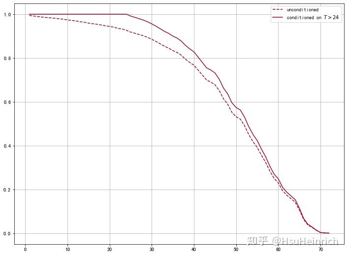
neg_rate = values[values['RemainingValue']image-20230206152201057如果用户生存曲线不超过0.5,预测的中位生存时间是inf,可以采用cph.predict_percentile(churn0,p=0.6)计算分为数存活时间预测的最大存活时间为tenure的最大值,即无法预测到观测截面时间后的生存情况。因此也可以将inf定义为最大值一些用户会在流失前被预测为流失,因此存在剩余生存时间为负。可以通过校准纠偏# 预测未流失客户的生存曲线
unconditioned_sf = cph.predict_survival_function(churn0)
# 校准
conditioned_sf = unconditioned_sf.apply(lambda c: (c / c.loc[df.loc[c.name, 'tenure']]).clip(upper=1))
# 绘制校准曲线
fig, ax = plt.subplots(figsize=(12,9))
subject = 7038
tenures = df_model['tenure'].loc[subject,] # 查询index的位置,非自然位置
unconditioned_sf[subject].plot(ls="--", color="#A60628", label="unconditioned")
conditioned_sf[subject].plot(color="#A60628", label="conditioned on $T>{:.0f}$".format(tenures))
ax.legend()
ax.grid() output_34_0 模型在10月-20月的预测效果较好模型应用预测剩余价值# 筛选未流失用户
churn0 = df_model.query("Churn == 0")
# 预测中位数生存时间
churn0_median_survive = cph.predict_median(churn0).rename('median_survive')
# 计算剩余价值=月消费*(预测中位数生存时间)-已存续时间
values = pd.concat([churn0_median_survive, churn0[['MonthlyCharges','tenure']]], axis=1)
values['RemainTenure'] = values['median_survive'] - values['tenure']
values['RemainingValue'] = values['MonthlyCharges'] * values['RemainTenure']
# 计算RemainingValue负值与inf的占比
inf_rate = values[values['RemainingValue']==float('inf')].shape[0]/values.shape[0]
neg_rate = values[values['RemainingValue']image-20230206152201057如果用户生存曲线不超过0.5,预测的中位生存时间是inf,可以采用cph.predict_percentile(churn0,p=0.6)计算分为数存活时间预测的最大存活时间为tenure的最大值,即无法预测到观测截面时间后的生存情况。因此也可以将inf定义为最大值一些用户会在流失前被预测为流失,因此存在剩余生存时间为负。可以通过校准纠偏# 预测未流失客户的生存曲线
unconditioned_sf = cph.predict_survival_function(churn0)
# 校准
conditioned_sf = unconditioned_sf.apply(lambda c: (c / c.loc[df.loc[c.name, 'tenure']]).clip(upper=1))
# 绘制校准曲线
fig, ax = plt.subplots(figsize=(12,9))
subject = 7038
tenures = df_model['tenure'].loc[subject,] # 查询index的位置,非自然位置
unconditioned_sf[subject].plot(ls="--", color="#A60628", label="unconditioned")
conditioned_sf[subject].plot(color="#A60628", label="conditioned on $T>{:.0f}$".format(tenures))
ax.legend()
ax.grid()
 output_40_0# 根据校准曲线纠偏
churn0_median_survive_new = median_survival_times(conditioned_sf)
values_new = pd.concat([churn0[['tenure','MonthlyCharges']], churn0_median_survive_new.T], axis=1)
values_new.rename(columns={0.5:'median_survive'}, inplace=True)
values_new['RemainTenure'] = values_new['median_survive'] - values_new['tenure']
values_new['RemainingValue'] = values_new['MonthlyCharges'] * values_new['RemainTenure']
# 计算RemainingValue负值与inf的占比
inf_rate = values_new[values_new['RemainingValue']==float('inf')].shape[0]/values_new.shape[0]
neg_rate = values_new[values_new['RemainingValue']image-20230206152222706剩余价值提升# 将之前的校准写成函数
def predict_median_func(churn0):
unconditioned_sf = cph.predict_survival_function(churn0)
conditioned_sf = unconditioned_sf.apply(lambda c: (c / c.loc[df.loc[c.name, 'tenure']]).clip(upper=1))
churn0_median_survive_new = median_survival_times(conditioned_sf).T
return churn0_median_survive_new
# 将月签合同提升至一年合同,若原先是两年合同则维持不变
tmp =df_model.loc[values_new.index,].copy()
tmp['Contract_One year'] = tmp.apply(lambda x: 1 if x['Contract_Two year'] == 0 else 0, axis=1)
values_new['contract_1y_tenure_pred'] = predict_median_func(tmp)
# 将月签合同或者一年合同提升至两年合同
tmp =df_model.loc[values_new.index,].copy()
tmp['Contract_Two year'] = 1
tmp['Contract_One year'] = 0
values_new['contract_2y_tenure_pred'] = predict_median_func(tmp)
# 提升在线安全服务
tmp =df_model.loc[values_new.index,].copy()
tmp['OnlineSecurity_Yes'] = 1
values_new['OnlineSecurity_tenure_pred'] = predict_median_func(tmp)
# 计算剩余价值
values_new['Contract_1y Diff'] = (values_new['contract_1y_tenure_pred'] - values_new['median_survive']) * values_new['MonthlyCharges']
values_new['Contract_2y Diff'] = (values_new['contract_2y_tenure_pred'] - values_new['median_survive']) * values_new['MonthlyCharges']
values_new['OnlineSecurity Diff'] = (values_new['OnlineSecurity_tenure_pred'] - values_new['median_survive']) * values_new['MonthlyCharges']
# 预览结果
values_new.head().T output_40_0# 根据校准曲线纠偏
churn0_median_survive_new = median_survival_times(conditioned_sf)
values_new = pd.concat([churn0[['tenure','MonthlyCharges']], churn0_median_survive_new.T], axis=1)
values_new.rename(columns={0.5:'median_survive'}, inplace=True)
values_new['RemainTenure'] = values_new['median_survive'] - values_new['tenure']
values_new['RemainingValue'] = values_new['MonthlyCharges'] * values_new['RemainTenure']
# 计算RemainingValue负值与inf的占比
inf_rate = values_new[values_new['RemainingValue']==float('inf')].shape[0]/values_new.shape[0]
neg_rate = values_new[values_new['RemainingValue']image-20230206152222706剩余价值提升# 将之前的校准写成函数
def predict_median_func(churn0):
unconditioned_sf = cph.predict_survival_function(churn0)
conditioned_sf = unconditioned_sf.apply(lambda c: (c / c.loc[df.loc[c.name, 'tenure']]).clip(upper=1))
churn0_median_survive_new = median_survival_times(conditioned_sf).T
return churn0_median_survive_new
# 将月签合同提升至一年合同,若原先是两年合同则维持不变
tmp =df_model.loc[values_new.index,].copy()
tmp['Contract_One year'] = tmp.apply(lambda x: 1 if x['Contract_Two year'] == 0 else 0, axis=1)
values_new['contract_1y_tenure_pred'] = predict_median_func(tmp)
# 将月签合同或者一年合同提升至两年合同
tmp =df_model.loc[values_new.index,].copy()
tmp['Contract_Two year'] = 1
tmp['Contract_One year'] = 0
values_new['contract_2y_tenure_pred'] = predict_median_func(tmp)
# 提升在线安全服务
tmp =df_model.loc[values_new.index,].copy()
tmp['OnlineSecurity_Yes'] = 1
values_new['OnlineSecurity_tenure_pred'] = predict_median_func(tmp)
# 计算剩余价值
values_new['Contract_1y Diff'] = (values_new['contract_1y_tenure_pred'] - values_new['median_survive']) * values_new['MonthlyCharges']
values_new['Contract_2y Diff'] = (values_new['contract_2y_tenure_pred'] - values_new['median_survive']) * values_new['MonthlyCharges']
values_new['OnlineSecurity Diff'] = (values_new['OnlineSecurity_tenure_pred'] - values_new['median_survive']) * values_new['MonthlyCharges']
# 预览结果
values_new.head().T
 image-20230206152247133# 客户基本信息
df.loc[0,]
customerID 7590-VHVEG
gender Female
SeniorCitizen 0
Partner Yes
Dependents No
tenure 1
PhoneService No
MultipleLines No phone service
InternetService DSL
OnlineSecurity No
OnlineBackup Yes
DeviceProtection No
TechSupport No
StreamingTV No
StreamingMovies No
Contract Month-to-month
PaperlessBilling Yes
PaymentMethod Electronic check
MonthlyCharges 29.85
TotalCharges 29.85
Churn 0
Name: 0, dtype: object0号客户基本信息:使用时长(tenure)1个月,没有OnlineSecurity,Contract为月签。月费为29.850号客户基本预测信息:预测27个月,剩余价值805.950号客户价值提升信息: 更换1年合同后,预测43个月,剩余价值较月签合同提升了447.75更换2年合同后,预测65个月,剩余价值较月签合同提升了1104.45添加OnlineSecurity后,预测31个月,剩余价值较月签合同提升了89.55 image-20230206152247133# 客户基本信息
df.loc[0,]
customerID 7590-VHVEG
gender Female
SeniorCitizen 0
Partner Yes
Dependents No
tenure 1
PhoneService No
MultipleLines No phone service
InternetService DSL
OnlineSecurity No
OnlineBackup Yes
DeviceProtection No
TechSupport No
StreamingTV No
StreamingMovies No
Contract Month-to-month
PaperlessBilling Yes
PaymentMethod Electronic check
MonthlyCharges 29.85
TotalCharges 29.85
Churn 0
Name: 0, dtype: object0号客户基本信息:使用时长(tenure)1个月,没有OnlineSecurity,Contract为月签。月费为29.850号客户基本预测信息:预测27个月,剩余价值805.950号客户价值提升信息: 更换1年合同后,预测43个月,剩余价值较月签合同提升了447.75更换2年合同后,预测65个月,剩余价值较月签合同提升了1104.45添加OnlineSecurity后,预测31个月,剩余价值较月签合同提升了89.55
|
 image-20230206152049606数据预处理df = raw_data.copy()
# 删除tenure=0(This model does not allow for non-positive durations)
df = df[df['tenure']>0]
# 转换成连续型变量
df['TotalCharges'] = pd.to_numeric(df.TotalCharges, errors='coerce')
# 填充缺失值
df['TotalCharges'].fillna(0, inplace=True)
# 转换成类别变量
df['SeniorCitizen'] = df['SeniorCitizen'].astype("str")
# 将是否流失转换为01分布
df['Churn'] = df['Churn'].map({'No':0,'Yes':1})
生存分析探索查看整体生存曲线fig, ax = plt.subplots(nrows=2, ncols=1, figsize=(12,10))
# 整体生存曲线
kmf = KaplanMeierFitter()
kmf.fit(df.tenure, # 代表生存时长
event_observed=df.Churn # 代表事件的终点
)
kmf.plot_survival_function(ax=ax[0], label='all')
ax[0].grid()
# 整体生存变化率
naf = NelsonAalenFitter()
naf.fit(df.tenure, event_observed=df.Churn)
naf.plot_hazard(ax=ax[1], bandwidth=20, label='all')
ax[1].grid()
plt.show()
image-20230206152049606数据预处理df = raw_data.copy()
# 删除tenure=0(This model does not allow for non-positive durations)
df = df[df['tenure']>0]
# 转换成连续型变量
df['TotalCharges'] = pd.to_numeric(df.TotalCharges, errors='coerce')
# 填充缺失值
df['TotalCharges'].fillna(0, inplace=True)
# 转换成类别变量
df['SeniorCitizen'] = df['SeniorCitizen'].astype("str")
# 将是否流失转换为01分布
df['Churn'] = df['Churn'].map({'No':0,'Yes':1})
生存分析探索查看整体生存曲线fig, ax = plt.subplots(nrows=2, ncols=1, figsize=(12,10))
# 整体生存曲线
kmf = KaplanMeierFitter()
kmf.fit(df.tenure, # 代表生存时长
event_observed=df.Churn # 代表事件的终点
)
kmf.plot_survival_function(ax=ax[0], label='all')
ax[0].grid()
# 整体生存变化率
naf = NelsonAalenFitter()
naf.fit(df.tenure, event_observed=df.Churn)
naf.plot_hazard(ax=ax[1], bandwidth=20, label='all')
ax[1].grid()
plt.show()
 output_8_0截至观察期(最大70个月),整体还有60%的用户未流失。不存在半衰期,即当用户流失达到50%的时间节点0-10个月用户流失加快,50-60个月的用户流失速率也有所提升# 缩短时间查看前20个月
t = np.linspace(0, 20, 21)
fig, ax = plt.subplots(nrows=2, ncols=1, figsize=(12,10))
# 整体生存曲线
kmf = KaplanMeierFitter()
kmf.fit(df.tenure, # 代表生存时长
event_observed=df.Churn, # 代表事件的终点
timeline=t
)
kmf.plot_survival_function(ax=ax[0], label='all')
# 整体生存变化率
naf = NelsonAalenFitter()
naf.fit(df.tenure, event_observed=df.Churn, timeline=t)
naf.plot_hazard(ax=ax[1], bandwidth=20, label='all')
plt.show()
output_8_0截至观察期(最大70个月),整体还有60%的用户未流失。不存在半衰期,即当用户流失达到50%的时间节点0-10个月用户流失加快,50-60个月的用户流失速率也有所提升# 缩短时间查看前20个月
t = np.linspace(0, 20, 21)
fig, ax = plt.subplots(nrows=2, ncols=1, figsize=(12,10))
# 整体生存曲线
kmf = KaplanMeierFitter()
kmf.fit(df.tenure, # 代表生存时长
event_observed=df.Churn, # 代表事件的终点
timeline=t
)
kmf.plot_survival_function(ax=ax[0], label='all')
# 整体生存变化率
naf = NelsonAalenFitter()
naf.fit(df.tenure, event_observed=df.Churn, timeline=t)
naf.plot_hazard(ax=ax[1], bandwidth=20, label='all')
plt.show()
 output_10_0第一个月是用户流失重灾时间前10个月中,前5个月流失速率加快查看单变量生存曲线差异# 连续变量分箱
combiner = toad.transform.Combiner()
combiner.fit(df[['MonthlyCharges','TotalCharges']], df['Churn'], method='chi', # 卡方分箱
min_samples=0.05)
df_t = combiner.transform(df)
# 筛选变量
obj_list = df_t.select_dtypes(include="object").columns[1:].to_list()
obj_list += ['MonthlyCharges','TotalCharges']
# 计算行列数
num_plots = len(obj_list)
num_cols = math.ceil(np.sqrt(num_plots))
num_rows = math.ceil(num_plots/num_cols)
cr = [d for d in itertools.product(range(num_rows),range(num_cols))]
# 绘制生存曲线
fig, ax = plt.subplots(nrows=num_rows, ncols=num_cols, figsize=(48,36))
for ind,feature in enumerate(obj_list):
for i in df_t[feature].unique():
# KaplanMeier检验
kmf=KaplanMeierFitter()
df_tmp = df_t.loc[df_t[feature] == i]
kmf.fit(df_tmp.tenure, # 代表生存时长
event_observed=df_tmp.Churn, # 代表事件的终点
label=i)
# 绘制生存曲线
kmf.plot_survival_function(ci_show=False,
ax = ax[cr[ind][0]][cr[ind][1]])
# 对数秩检验,得到p值
p_value = multivariate_logrank_test(event_durations = df_t.tenure, # 代表生存时长
groups=df_t[feature], # 代表检验的组别
event_observed=df_t.Churn # 代表事件的终点
).p_value
p_value_text = ['p-value < 0.001' if p_value output_13_0验证多分类单变量生存曲线差异# 查看多分类变量的组间差异:以PaymentMethod为例
fig, ax = plt.subplots(figsize=(10,6))
feature = 'PaymentMethod'
for i in df_t[feature].unique():
# KaplanMeier检验
kmf=KaplanMeierFitter()
df_tmp = df_t.loc[df_t[feature] == i]
kmf.fit(df_tmp.tenure, # 代表生存时长
event_observed=df_tmp.Churn, # 代表事件的终点
label=i)
# 绘制生存曲线
kmf.plot_survival_function(ci_show=False,
ax = ax)
# 对数秩检验,得到p值
p_value = multivariate_logrank_test(event_durations = df_t.tenure, # 代表生存时长
groups=df_t[feature], # 代表检验的组别
event_observed=df_t.Churn # 代表事件的终点
).p_value
p_value_text = ['p-value < 0.001' if p_value image-20221221185003629生存曲线表明PaymentMethod存在组间显著差异检验表明除了Bank transfer (automatic)与Credit card (automatic)不存在显著差异,其余组间均显著差异交互变量的生存曲线# 以性别gender为例,查看与其他变量交互后,gender的流失情况是否存在显著差异
for feature in obj_list:
for i in df_t[feature].unique():
df_tmp = df_t.loc[df_t[feature] == i]
p_value = multivariate_logrank_test(event_durations = df_tmp.tenure,
groups=df_tmp.gender,
event_observed=df_tmp.Churn
).p_value
if p_value output_20_0 在Credit card (automatic)客户中,Female更容易流失 特征工程# 特征工程
df_model = pd.get_dummies(df.iloc[:,1:], drop_first=True) # 剔除客户ID,并对类别变量进行哑变量处理(剔除首列防止虚拟变量陷阱)
# 拆分训练集
train, test = train_test_split(df_model, test_size=0.2)
数据建模模型拟合# 模型拟合
cph = CoxPHFitter(penalizer = 0.01)
cph.fit(train, duration_col='tenure', event_col='Churn')
cph.print_summary(decimals=1)
modellifelines.CoxPHFitterduration col'tenure'event col'Churn'penalizer0.01l1 ratio0baseline estimationbreslownumber of observations5625number of events observed1500partial log-likelihood-10138.3time fit was run2022-09-16 15:52:24 UTC
output_10_0第一个月是用户流失重灾时间前10个月中,前5个月流失速率加快查看单变量生存曲线差异# 连续变量分箱
combiner = toad.transform.Combiner()
combiner.fit(df[['MonthlyCharges','TotalCharges']], df['Churn'], method='chi', # 卡方分箱
min_samples=0.05)
df_t = combiner.transform(df)
# 筛选变量
obj_list = df_t.select_dtypes(include="object").columns[1:].to_list()
obj_list += ['MonthlyCharges','TotalCharges']
# 计算行列数
num_plots = len(obj_list)
num_cols = math.ceil(np.sqrt(num_plots))
num_rows = math.ceil(num_plots/num_cols)
cr = [d for d in itertools.product(range(num_rows),range(num_cols))]
# 绘制生存曲线
fig, ax = plt.subplots(nrows=num_rows, ncols=num_cols, figsize=(48,36))
for ind,feature in enumerate(obj_list):
for i in df_t[feature].unique():
# KaplanMeier检验
kmf=KaplanMeierFitter()
df_tmp = df_t.loc[df_t[feature] == i]
kmf.fit(df_tmp.tenure, # 代表生存时长
event_observed=df_tmp.Churn, # 代表事件的终点
label=i)
# 绘制生存曲线
kmf.plot_survival_function(ci_show=False,
ax = ax[cr[ind][0]][cr[ind][1]])
# 对数秩检验,得到p值
p_value = multivariate_logrank_test(event_durations = df_t.tenure, # 代表生存时长
groups=df_t[feature], # 代表检验的组别
event_observed=df_t.Churn # 代表事件的终点
).p_value
p_value_text = ['p-value < 0.001' if p_value output_13_0验证多分类单变量生存曲线差异# 查看多分类变量的组间差异:以PaymentMethod为例
fig, ax = plt.subplots(figsize=(10,6))
feature = 'PaymentMethod'
for i in df_t[feature].unique():
# KaplanMeier检验
kmf=KaplanMeierFitter()
df_tmp = df_t.loc[df_t[feature] == i]
kmf.fit(df_tmp.tenure, # 代表生存时长
event_observed=df_tmp.Churn, # 代表事件的终点
label=i)
# 绘制生存曲线
kmf.plot_survival_function(ci_show=False,
ax = ax)
# 对数秩检验,得到p值
p_value = multivariate_logrank_test(event_durations = df_t.tenure, # 代表生存时长
groups=df_t[feature], # 代表检验的组别
event_observed=df_t.Churn # 代表事件的终点
).p_value
p_value_text = ['p-value < 0.001' if p_value image-20221221185003629生存曲线表明PaymentMethod存在组间显著差异检验表明除了Bank transfer (automatic)与Credit card (automatic)不存在显著差异,其余组间均显著差异交互变量的生存曲线# 以性别gender为例,查看与其他变量交互后,gender的流失情况是否存在显著差异
for feature in obj_list:
for i in df_t[feature].unique():
df_tmp = df_t.loc[df_t[feature] == i]
p_value = multivariate_logrank_test(event_durations = df_tmp.tenure,
groups=df_tmp.gender,
event_observed=df_tmp.Churn
).p_value
if p_value output_20_0 在Credit card (automatic)客户中,Female更容易流失 特征工程# 特征工程
df_model = pd.get_dummies(df.iloc[:,1:], drop_first=True) # 剔除客户ID,并对类别变量进行哑变量处理(剔除首列防止虚拟变量陷阱)
# 拆分训练集
train, test = train_test_split(df_model, test_size=0.2)
数据建模模型拟合# 模型拟合
cph = CoxPHFitter(penalizer = 0.01)
cph.fit(train, duration_col='tenure', event_col='Churn')
cph.print_summary(decimals=1)
modellifelines.CoxPHFitterduration col'tenure'event col'Churn'penalizer0.01l1 ratio0baseline estimationbreslownumber of observations5625number of events observed1500partial log-likelihood-10138.3time fit was run2022-09-16 15:52:24 UTC image-20221221185924375Concordance=0.9,模型拟合不错。Concordance Index是AUC的推广,值越接近1效果越好系数为正则表示该变量促进流失,系数为负表示该变量防止流失显著影响的为p0.05].index)
train_s = train.drop(drop_col, axis=1)
test_s = test.drop(drop_col, axis=1)
# 重新拟合
cph = CoxPHFitter(penalizer = 0.01)
cph.fit(train_s, duration_col='tenure', event_col='Churn')
cph.print_summary(decimals=1)
image-20221221185924375Concordance=0.9,模型拟合不错。Concordance Index是AUC的推广,值越接近1效果越好系数为正则表示该变量促进流失,系数为负表示该变量防止流失显著影响的为p0.05].index)
train_s = train.drop(drop_col, axis=1)
test_s = test.drop(drop_col, axis=1)
# 重新拟合
cph = CoxPHFitter(penalizer = 0.01)
cph.fit(train_s, duration_col='tenure', event_col='Churn')
cph.print_summary(decimals=1)
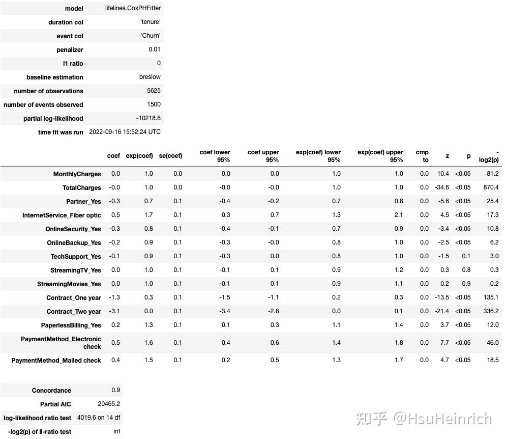 image-20221221190131160特征重要性# 特征重要性
fig,ax = plt.subplots(figsize=(12,9))
cph.plot(ax=ax)
plt.show()
image-20221221190131160特征重要性# 特征重要性
fig,ax = plt.subplots(figsize=(12,9))
cph.plot(ax=ax)
plt.show()
 output_27_0加速流失的变量有:InternetService_Fiber optic、PaymentMethod_Mailed check等防止流失的变量有:Contract_Two year、Contract_One year等风险观察# 累积风险曲线
fig,ax = plt.subplots(nrows=2, ncols=1, figsize=(10,12))
cph.baseline_cumulative_hazard_.plot(ax=ax[0])
# 各时间节点的风险曲线
cph.baseline_hazard_.plot(ax=ax[1])
plt.show()
output_27_0加速流失的变量有:InternetService_Fiber optic、PaymentMethod_Mailed check等防止流失的变量有:Contract_Two year、Contract_One year等风险观察# 累积风险曲线
fig,ax = plt.subplots(nrows=2, ncols=1, figsize=(10,12))
cph.baseline_cumulative_hazard_.plot(ax=ax[0])
# 各时间节点的风险曲线
cph.baseline_hazard_.plot(ax=ax[1])
plt.show()
 output_29_0 在60个月以后流失风险明显提高模型评估# 模型校准性
fig,ax = plt.subplots(figsize=(12,9))
survival_probability_calibration(cph, test_s, t0=50, ax=ax)
ax.grid()
ICI = 0.05854302858419381
E50 = 0.021989969295193035
output_29_0 在60个月以后流失风险明显提高模型评估# 模型校准性
fig,ax = plt.subplots(figsize=(12,9))
survival_probability_calibration(cph, test_s, t0=50, ax=ax)
ax.grid()
ICI = 0.05854302858419381
E50 = 0.021989969295193035 output_32_1x轴为预测的流失概率,y轴为观测的流失概率以50个月为例,模型与基准值(对角线)偏离较大,且一直高估了用户的流失情况建议样本均衡处理,剔除具有相关性的特征等# 使用brier score观测校准距离:Brier分数对于一组预测值越低,预测校准越好
loss_dict = {}
for i in range(1,73):
score = brier_score_loss(
test_s.Churn,
1 - np.array(cph.predict_survival_function(test_s).loc[i]),
pos_label=1 )
loss_dict[i] = [score]
loss_df = pd.DataFrame(loss_dict).T
fig, ax = plt.subplots(figsize=(12,9))
ax.plot(loss_df.index, loss_df)
ax.set(xlabel='Prediction Time', ylabel='Calibration Loss', title='Cox PH Model Calibration Loss / Time')
ax.grid()
output_32_1x轴为预测的流失概率,y轴为观测的流失概率以50个月为例,模型与基准值(对角线)偏离较大,且一直高估了用户的流失情况建议样本均衡处理,剔除具有相关性的特征等# 使用brier score观测校准距离:Brier分数对于一组预测值越低,预测校准越好
loss_dict = {}
for i in range(1,73):
score = brier_score_loss(
test_s.Churn,
1 - np.array(cph.predict_survival_function(test_s).loc[i]),
pos_label=1 )
loss_dict[i] = [score]
loss_df = pd.DataFrame(loss_dict).T
fig, ax = plt.subplots(figsize=(12,9))
ax.plot(loss_df.index, loss_df)
ax.set(xlabel='Prediction Time', ylabel='Calibration Loss', title='Cox PH Model Calibration Loss / Time')
ax.grid()
 output_34_0 模型在10月-20月的预测效果较好模型应用预测剩余价值# 筛选未流失用户
churn0 = df_model.query("Churn == 0")
# 预测中位数生存时间
churn0_median_survive = cph.predict_median(churn0).rename('median_survive')
# 计算剩余价值=月消费*(预测中位数生存时间)-已存续时间
values = pd.concat([churn0_median_survive, churn0[['MonthlyCharges','tenure']]], axis=1)
values['RemainTenure'] = values['median_survive'] - values['tenure']
values['RemainingValue'] = values['MonthlyCharges'] * values['RemainTenure']
# 计算RemainingValue负值与inf的占比
inf_rate = values[values['RemainingValue']==float('inf')].shape[0]/values.shape[0]
neg_rate = values[values['RemainingValue']image-20230206152201057如果用户生存曲线不超过0.5,预测的中位生存时间是inf,可以采用cph.predict_percentile(churn0,p=0.6)计算分为数存活时间预测的最大存活时间为tenure的最大值,即无法预测到观测截面时间后的生存情况。因此也可以将inf定义为最大值一些用户会在流失前被预测为流失,因此存在剩余生存时间为负。可以通过校准纠偏# 预测未流失客户的生存曲线
unconditioned_sf = cph.predict_survival_function(churn0)
# 校准
conditioned_sf = unconditioned_sf.apply(lambda c: (c / c.loc[df.loc[c.name, 'tenure']]).clip(upper=1))
# 绘制校准曲线
fig, ax = plt.subplots(figsize=(12,9))
subject = 7038
tenures = df_model['tenure'].loc[subject,] # 查询index的位置,非自然位置
unconditioned_sf[subject].plot(ls="--", color="#A60628", label="unconditioned")
conditioned_sf[subject].plot(color="#A60628", label="conditioned on $T>{:.0f}$".format(tenures))
ax.legend()
ax.grid()
output_34_0 模型在10月-20月的预测效果较好模型应用预测剩余价值# 筛选未流失用户
churn0 = df_model.query("Churn == 0")
# 预测中位数生存时间
churn0_median_survive = cph.predict_median(churn0).rename('median_survive')
# 计算剩余价值=月消费*(预测中位数生存时间)-已存续时间
values = pd.concat([churn0_median_survive, churn0[['MonthlyCharges','tenure']]], axis=1)
values['RemainTenure'] = values['median_survive'] - values['tenure']
values['RemainingValue'] = values['MonthlyCharges'] * values['RemainTenure']
# 计算RemainingValue负值与inf的占比
inf_rate = values[values['RemainingValue']==float('inf')].shape[0]/values.shape[0]
neg_rate = values[values['RemainingValue']image-20230206152201057如果用户生存曲线不超过0.5,预测的中位生存时间是inf,可以采用cph.predict_percentile(churn0,p=0.6)计算分为数存活时间预测的最大存活时间为tenure的最大值,即无法预测到观测截面时间后的生存情况。因此也可以将inf定义为最大值一些用户会在流失前被预测为流失,因此存在剩余生存时间为负。可以通过校准纠偏# 预测未流失客户的生存曲线
unconditioned_sf = cph.predict_survival_function(churn0)
# 校准
conditioned_sf = unconditioned_sf.apply(lambda c: (c / c.loc[df.loc[c.name, 'tenure']]).clip(upper=1))
# 绘制校准曲线
fig, ax = plt.subplots(figsize=(12,9))
subject = 7038
tenures = df_model['tenure'].loc[subject,] # 查询index的位置,非自然位置
unconditioned_sf[subject].plot(ls="--", color="#A60628", label="unconditioned")
conditioned_sf[subject].plot(color="#A60628", label="conditioned on $T>{:.0f}$".format(tenures))
ax.legend()
ax.grid()
 output_40_0# 根据校准曲线纠偏
churn0_median_survive_new = median_survival_times(conditioned_sf)
values_new = pd.concat([churn0[['tenure','MonthlyCharges']], churn0_median_survive_new.T], axis=1)
values_new.rename(columns={0.5:'median_survive'}, inplace=True)
values_new['RemainTenure'] = values_new['median_survive'] - values_new['tenure']
values_new['RemainingValue'] = values_new['MonthlyCharges'] * values_new['RemainTenure']
# 计算RemainingValue负值与inf的占比
inf_rate = values_new[values_new['RemainingValue']==float('inf')].shape[0]/values_new.shape[0]
neg_rate = values_new[values_new['RemainingValue']image-20230206152222706剩余价值提升# 将之前的校准写成函数
def predict_median_func(churn0):
unconditioned_sf = cph.predict_survival_function(churn0)
conditioned_sf = unconditioned_sf.apply(lambda c: (c / c.loc[df.loc[c.name, 'tenure']]).clip(upper=1))
churn0_median_survive_new = median_survival_times(conditioned_sf).T
return churn0_median_survive_new
# 将月签合同提升至一年合同,若原先是两年合同则维持不变
tmp =df_model.loc[values_new.index,].copy()
tmp['Contract_One year'] = tmp.apply(lambda x: 1 if x['Contract_Two year'] == 0 else 0, axis=1)
values_new['contract_1y_tenure_pred'] = predict_median_func(tmp)
# 将月签合同或者一年合同提升至两年合同
tmp =df_model.loc[values_new.index,].copy()
tmp['Contract_Two year'] = 1
tmp['Contract_One year'] = 0
values_new['contract_2y_tenure_pred'] = predict_median_func(tmp)
# 提升在线安全服务
tmp =df_model.loc[values_new.index,].copy()
tmp['OnlineSecurity_Yes'] = 1
values_new['OnlineSecurity_tenure_pred'] = predict_median_func(tmp)
# 计算剩余价值
values_new['Contract_1y Diff'] = (values_new['contract_1y_tenure_pred'] - values_new['median_survive']) * values_new['MonthlyCharges']
values_new['Contract_2y Diff'] = (values_new['contract_2y_tenure_pred'] - values_new['median_survive']) * values_new['MonthlyCharges']
values_new['OnlineSecurity Diff'] = (values_new['OnlineSecurity_tenure_pred'] - values_new['median_survive']) * values_new['MonthlyCharges']
# 预览结果
values_new.head().T
output_40_0# 根据校准曲线纠偏
churn0_median_survive_new = median_survival_times(conditioned_sf)
values_new = pd.concat([churn0[['tenure','MonthlyCharges']], churn0_median_survive_new.T], axis=1)
values_new.rename(columns={0.5:'median_survive'}, inplace=True)
values_new['RemainTenure'] = values_new['median_survive'] - values_new['tenure']
values_new['RemainingValue'] = values_new['MonthlyCharges'] * values_new['RemainTenure']
# 计算RemainingValue负值与inf的占比
inf_rate = values_new[values_new['RemainingValue']==float('inf')].shape[0]/values_new.shape[0]
neg_rate = values_new[values_new['RemainingValue']image-20230206152222706剩余价值提升# 将之前的校准写成函数
def predict_median_func(churn0):
unconditioned_sf = cph.predict_survival_function(churn0)
conditioned_sf = unconditioned_sf.apply(lambda c: (c / c.loc[df.loc[c.name, 'tenure']]).clip(upper=1))
churn0_median_survive_new = median_survival_times(conditioned_sf).T
return churn0_median_survive_new
# 将月签合同提升至一年合同,若原先是两年合同则维持不变
tmp =df_model.loc[values_new.index,].copy()
tmp['Contract_One year'] = tmp.apply(lambda x: 1 if x['Contract_Two year'] == 0 else 0, axis=1)
values_new['contract_1y_tenure_pred'] = predict_median_func(tmp)
# 将月签合同或者一年合同提升至两年合同
tmp =df_model.loc[values_new.index,].copy()
tmp['Contract_Two year'] = 1
tmp['Contract_One year'] = 0
values_new['contract_2y_tenure_pred'] = predict_median_func(tmp)
# 提升在线安全服务
tmp =df_model.loc[values_new.index,].copy()
tmp['OnlineSecurity_Yes'] = 1
values_new['OnlineSecurity_tenure_pred'] = predict_median_func(tmp)
# 计算剩余价值
values_new['Contract_1y Diff'] = (values_new['contract_1y_tenure_pred'] - values_new['median_survive']) * values_new['MonthlyCharges']
values_new['Contract_2y Diff'] = (values_new['contract_2y_tenure_pred'] - values_new['median_survive']) * values_new['MonthlyCharges']
values_new['OnlineSecurity Diff'] = (values_new['OnlineSecurity_tenure_pred'] - values_new['median_survive']) * values_new['MonthlyCharges']
# 预览结果
values_new.head().T
 image-20230206152247133# 客户基本信息
df.loc[0,]
customerID 7590-VHVEG
gender Female
SeniorCitizen 0
Partner Yes
Dependents No
tenure 1
PhoneService No
MultipleLines No phone service
InternetService DSL
OnlineSecurity No
OnlineBackup Yes
DeviceProtection No
TechSupport No
StreamingTV No
StreamingMovies No
Contract Month-to-month
PaperlessBilling Yes
PaymentMethod Electronic check
MonthlyCharges 29.85
TotalCharges 29.85
Churn 0
Name: 0, dtype: object0号客户基本信息:使用时长(tenure)1个月,没有OnlineSecurity,Contract为月签。月费为29.850号客户基本预测信息:预测27个月,剩余价值805.950号客户价值提升信息: 更换1年合同后,预测43个月,剩余价值较月签合同提升了447.75更换2年合同后,预测65个月,剩余价值较月签合同提升了1104.45添加OnlineSecurity后,预测31个月,剩余价值较月签合同提升了89.55
image-20230206152247133# 客户基本信息
df.loc[0,]
customerID 7590-VHVEG
gender Female
SeniorCitizen 0
Partner Yes
Dependents No
tenure 1
PhoneService No
MultipleLines No phone service
InternetService DSL
OnlineSecurity No
OnlineBackup Yes
DeviceProtection No
TechSupport No
StreamingTV No
StreamingMovies No
Contract Month-to-month
PaperlessBilling Yes
PaymentMethod Electronic check
MonthlyCharges 29.85
TotalCharges 29.85
Churn 0
Name: 0, dtype: object0号客户基本信息:使用时长(tenure)1个月,没有OnlineSecurity,Contract为月签。月费为29.850号客户基本预测信息:预测27个月,剩余价值805.950号客户价值提升信息: 更换1年合同后,预测43个月,剩余价值较月签合同提升了447.75更换2年合同后,预测65个月,剩余价值较月签合同提升了1104.45添加OnlineSecurity后,预测31个月,剩余价值较月签合同提升了89.55