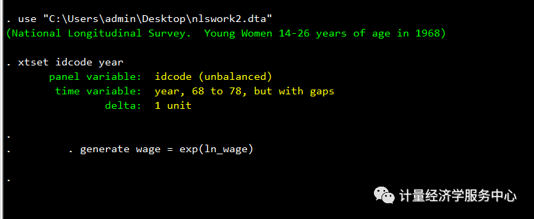
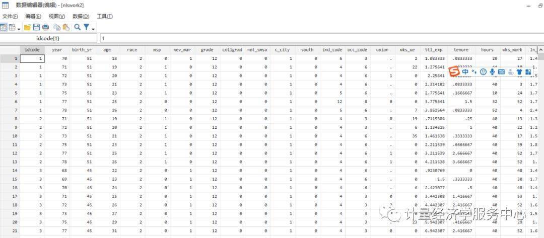
lags(#) ：定义pvar模型的最大滞后期，默认滞后期为1

exog(varlist) ：表示定义在PVAR模型中的内生变量列表

fod and fd：用来指定如何消除面板的固定效果。fod指定使用正向正交偏差或Helmert变换来消除面板固定效应，fod是默认选项。fd规定了使用一阶差分而不是正向正交偏差来消除特定于面板的固定效应。

td：表示减去模型中每个变量在估计之前的横截面均值。这可以用于在任何其他转换之前从所有变量中删除固定时间的效果。

gmmstyle指定使用Holtz-Eakin、Newey和Rosen(1988)提出的“GMM-style”工具。

gmmopts(options)覆盖pvar运行的默认gmm选项。可以使用depvarlist中的变量名作为方程名分别访问模型中的每个方程。

vce(vcetype[， independent])指定报告的标准误差类型

level(#)指定用于报告置信区间的置信水平(以百分比表示)。默认值是level(95)或按set level设置。

noprint：不汇报系数表

2、pvarsoc

pvarsoc提供各种简要措施，以帮助面板VAR模型的选择。它报告了模型总体决定系数，Hansen (1982) J统计量和相应的p值，以及Andrews和Lu(2001)基于J统计量制定的弯矩模型选择准则。Andrew和Lu的准则都是基于Hansen’s J统计量，它要求模型中的moment conditions数量大于内生变量的数量。

语法选项为：

maxlag(#)指定获得统计信息的最大滞后顺序。

pinstlag(numlist) specifies that the numlist-th lag from the highest lag order of depvarlist specified in the panel VAR model implemented using pvar be used. This option cannot be specified with the option

pvaropts(instlag(numlist)). pvaropts(options) passes arguments to pvar. All arguments specified in options are passed to and used by pvar in estimation.

3、pvargranger

pvargranger对面板VAR模型的每个方程进行Granger causality Wald tests.

estimate (estname)请求pvargranger使用之前获得的一组保存为estname的面板VAR估计。默认情况下，pvargranger使用活动(即最新)结果。

4、pvarstable

后估计命令pvarstable通过计算估计模型各特征值的向量来检查面板VAR估计的稳定性条件。Lutkepohl(2005)和Hamilton(1994)都表明，如果所有的伴随矩阵的向量都严格小于1，则VAR模型是稳定的。稳定性为估计脉冲响应函数和预测误差方差分解提供了已知的解释。

5、 pvarirf

后估计命令pvarirf计算并绘制脉冲响应函数(IRF)。根据蒙特卡罗估计的面板VAR模型，采用高斯逼近的方法估计置信度。正交化的IRF基于Cholesky分解，累积的IRF也可以使用pvarirf计算。

3

面板向量自回归PVAR操作应用

案例介绍1：

我们通过分析年工作时间和小时收入之间的关系来说明pvar命令集的使用，Holtz-Eakin, Newey和Rosen(1988)在他们关于面板向量自回归的开创性论文中分析了这一关系。为了将我们的新程序与Stata内置的var命令集进行比较，我们还将新的pvar命令集应用于Lutkephol(1993)的 West Germany 时间序列数据。

数据介绍：

我们使用了Stata提供的1968年至1978年全国纵向调查中14-26岁女性的子样本。我们的子样本包括2039名女性，她们在至少三轮调查中报告了工资(工资)和年度工作时间(小时)，其中两轮调查是连续进行的。Holtz-Eakin等人使用了相同的调查，但不同的时间段和不同的工作人员子样本，因此结果可能不是直接可比的。使用前四个滞后时间和工资作为工具，使用pvarsoc计算一到三阶面板VAR模型选择。

1、导入数据

2、查看数据如下：

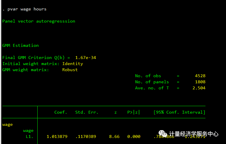
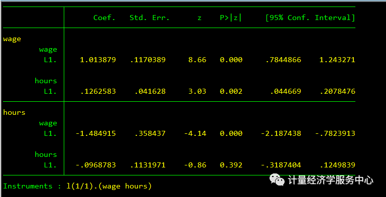
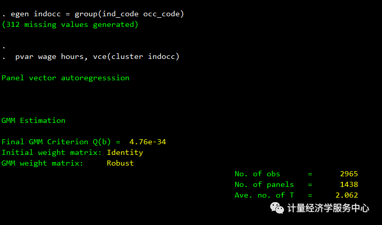
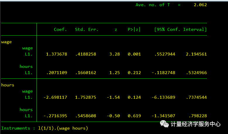
3、Helmert变换拟合面板VAR模型，滞后期选择默认的

结果为：

4、与上面相同，但是标准误按行业分类

结果为：

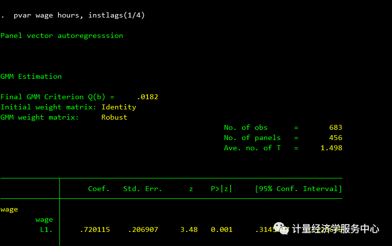
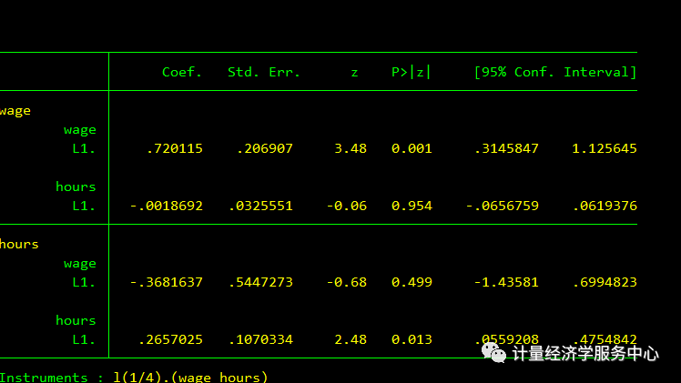
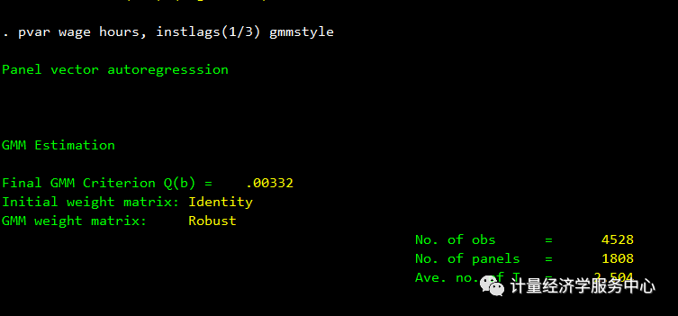
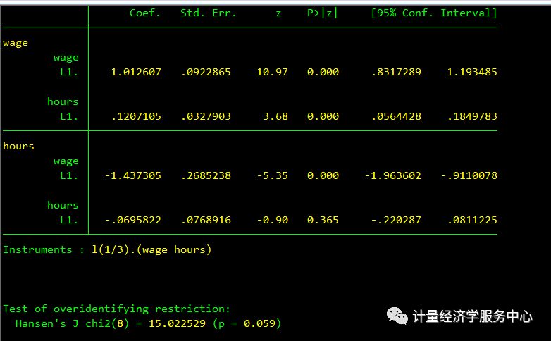
5、 Same as first but use the first four lags as instruments

结果为：

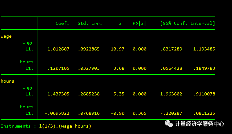
6、 use GMM-style instruments

结果为：

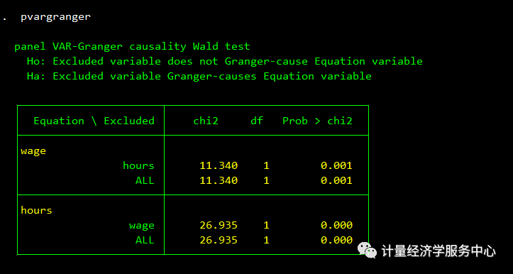
虽然可以从上面的pvar输出中推断出一阶面板变量的格兰杰因果关系，但是我们仍然使用pvargranger作为例子来执行测试。下面的格兰杰因果检验结果表明，在通常的信心水平下，工资格兰杰导致工作时间，而工作时间格兰杰导致工资，与Holtz-Eakin等人的发现类似。

7、格兰杰检验

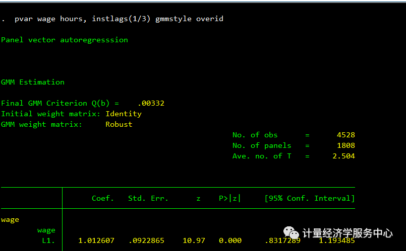
8、 Same as above but report overidentification test

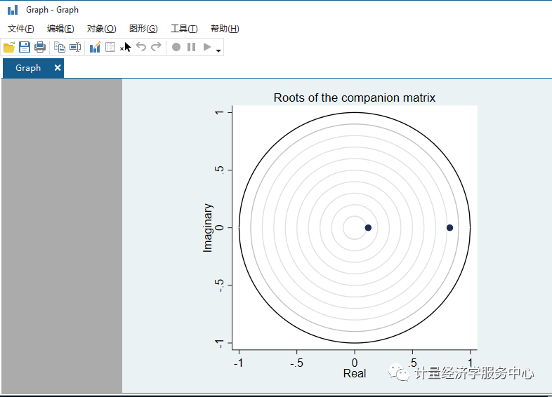
面板向量自回归模型估计本身很少被解释。在实践中，研究人员往往对各内生变量的外生变化对面板VAR系统中其他变量的影响感兴趣。然而，在估计脉冲响应函数(IRF)和预测误差方差分解(FEVD)之前，我们首先检查估计的面板变量的稳定性条件。得到的特征值表和图证实了估计是稳定的。

9、 稳定性检验

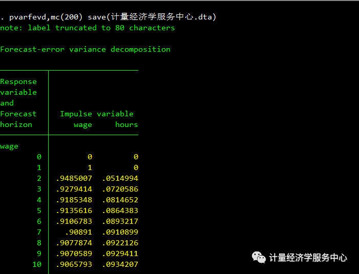
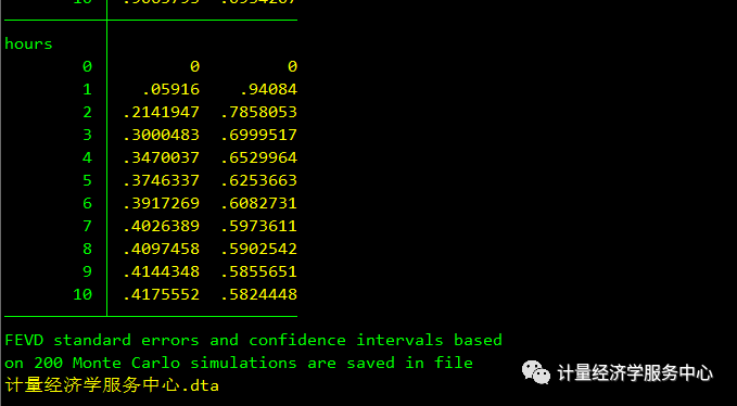
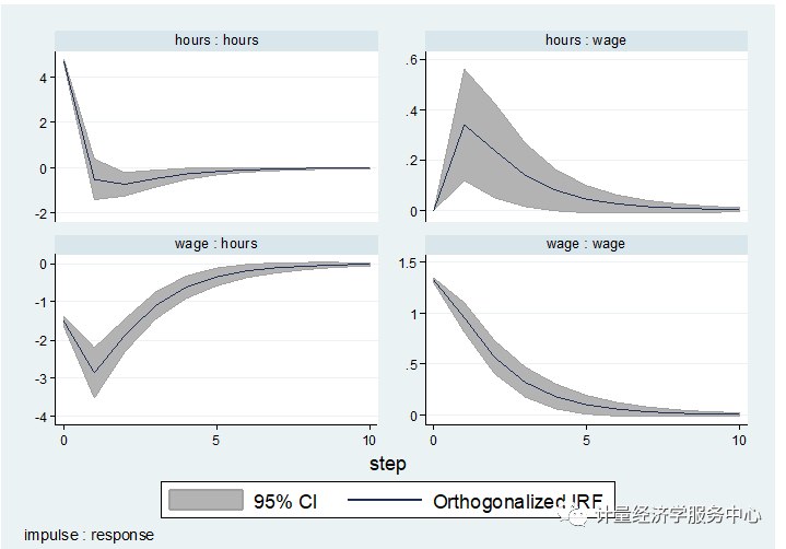
根据Holtz-Eakin等人的理论阐述，我们认为，工资水平的冲击直接影响同期的工作时间，而当前的工作努力只影响未来的工资。利用这个因果顺序，我们计算了使用pvarirf的隐含IRF和使用pvarfevd的隐含FEVD。在估计模型的基础上，使用200个蒙特卡罗图计算IRF置信区间。FEVD估计值的标准误差和置信区间同样可用，但这里没有显示，以节省空间。

10、pvarfevd

11、pvarirf

根据FEVD的估计，在我们的例子中，女性工作时间的变化中有40%可以用她们的工资来解释。另一方面，工作时间只能解释女性未来工资变化的5%。就水平而言，IRF图显示，对实际工资的正面冲击会导致工作努力减少，这意味着样本中的女性劳动力供应会向后弯曲。值得注意的是，当前工作努力的冲击对工作时间和工资都有积极但短暂的影响。另一方面，当前冲击对工资的影响对未来工资有持续的积极影响。

4

参考资料

Michael R.M. Abrigo and Inessa Love，Estimation of Panel Vector Autoregression in Stata: a Package of Programs

Akaike, H. (1969). Fitting autoregressive models for prediction. Annals of the Institute of StatisticalMathematics, 21, 243-247.

Akaike, H. (1977). On entropy maximization principle. In:Krishnaiah, P.R. (Ed.), Applications ofStatistics. Amsterdam: North-Holland.

Andrews, D.W.K. and B. Lu (2001). Consistent model and momentselection procedures for GMM estimation with application to dynamic panel datamodels. Journal of Econometrics,101(1), 123-164.

Arellano, M. and O. Bover (1995). Another look at the instrumentalvariable estimation of error-components model. Journal of Econometrics, 68(1), 29-51.

Bun, M.J.G. and M.A. Carree (2005). Bias-corrected estimation indynamic panel data models. Journal ofBusiness & Economic Statistics, 23(2), 200-210.

Canova, F. and M. Ciccarelli (2013). Panel vector autoregressivemodels: A survey. Advance in Econometrics,32,

Carpenter, S. and S. Demiralp (2012). Money, reserves, and thetransmission of monetary policy: Does the money multiplier exist? Journal of Macroeconomics, 34(1), 59-75.

Everaert, G. and L. Pozzi (2007). Bootstrap-based correction fordynamic panels. Journal of EconomicDynamics and Control, 31(4), 1160-1184.

Granger, C.W.J. (1969). Investigating causal relations by econometricmodels and cross-spectral methods. Econometrica,37(3), 424-438.

Hamilton, J.D. (1994). Time Series Analysis. Princeton: PrincetonUniversity Press.

Hannan, E.J. and B.G. Quinn (1979). The determination of the orderof an autoregression. Journal of theRoyal Statistical Society, Series B, 41(2), 190-195.

Hansen, L.P. (1982). Large sample properties of generalized methodof moments estimators. Econometrica,50(4), 1029-1054.

Head, H. H. Lloyd-Ellis and H. Sun (2015). Search, liquidity, andthe dynamics of house prices and construction. The American Economic Review, 104(4), 1172-1210.

Holtz-Eakin, D., W. Newey and H.S. Rosen (1988). Estimating vectorautoregressions with panel data. Econometrica,56(6), 1371-1395.

Judson, R.A., and A.L. Owen. 1999. Estimating dynamic panel datamodels: A guide for macroeconomists. EconomicsLetters, 65(1), 9-15.

Kiviet, J.F. (1995). On bias, inconsistency, and efficiency ofvarious estimators in dynamic panel data models. Journal of Econometrics, 68(1), 53-78.

Love, I. and L. Zicchino (2006). Financial development and dynamicinvestment behavior: Evidence from panel VAR. The Quarterly Review of Economics and Finance, 46(2), 190-210.

Lutkepohl, H. (1993). Introduction to Multiple Time Series Analysis,2nd Ed. New York: Springer.

Lutkepohl, H. (2005). New Introduction to Multiple Time SeriesAnalysis. New York: Springer.

Mora, N. and A. Logan (2012). Shocks to bank capital: Evidence fromUK banks at home and away. AppliedEconomics, 44(9), 1103-1119.

Neumann, T.C., P.V. Fishback and S. Kantor (2010). The dynamics ofrelief spending and the private urban market during the New Deal. The Journal of Economic History, 70(1)195-220.

Nickell,S.J. (1981). Biases in dynamic models with fixed effects. Econometrica, 49(6), 1417-1426.

Risannen, J. (1978). Modeling by shortest data deion. Automatica, 14(5), 465-471.

Roodman, D. (2009). How to doxtabond2: An introduction to difference and system GMM in Stata. The Stata Journal, 9(1), 86-139.

Schwarz, G. (1978). Estimating the dimension of a model. Annals of Statistics, 6(2), 461-464.

Sims, C.A. (1980). Macroeconomics and reality. Econometrica, 48(1), 1-48.

◆◆◆◆

点击上图查看：

《初级计量经济学及Stata应用：Stata从入门到进阶》

点击上图查看：

《零基础|轻松搞定空间计量： 空间计量及GeoDa、Stata应用》

点击上图查看：

计量经济学小白必修课--网课《高级计量经济学及Eviews应用》震撼上架！

点击上图查看：

空间计量及Matlab应用课程 返回搜狐，查看更多