💥💥💞💞欢迎来到本博客❤️❤️💥💥

🏆博主优势：🌞🌞🌞博客内容尽量做到思维缜密，逻辑清晰，为了方便读者。

⛳️座右铭：行百里者，半于九十。

📋📋📋本文目录如下：🎁🎁🎁

目录

💥1 概述

📚2 运行结果

🎉3 参考文献

🌈4 Matlab代码实现

文献来源：

@article{gu2022multi,   title={Multi-level Adaptation for Automatic Landing with Engine Failure under Turbulent Weather},   author={Gu, Haotian and Jafarnejadsani, Hamidreza},   journal={arXiv preprint arXiv:2209.04132},   year={2022} }

运行MASC示例 1.打开定义引擎输出纬度、经度和高度的程序。然后首先把飞机放到发动机坏掉的地方。然后单击右上角的停止按钮×平面窗口的角落。 2在故障位置配置块中设置发动机输出全局位置

3.在simulink框架中设置机场坐标 4.单击运行按钮，首先启动模拟模型。  

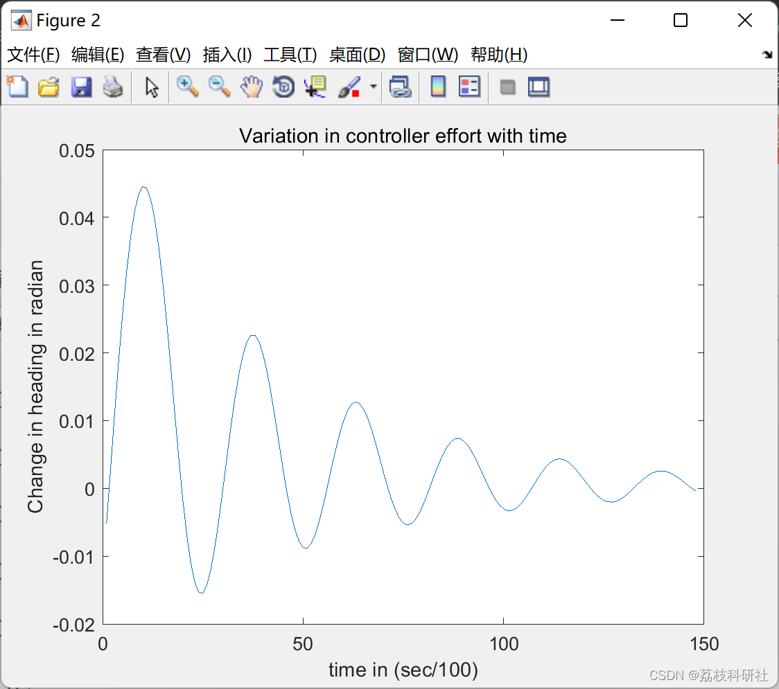
部分代码：

tic e = zeros(1,8000); c = zeros(1,8000); aileron_e = zeros(1,8000); psi_ref = zeros(1,8000); gamma_ref = zeros(1,8000); %% This function is for testing for converge to planned straight line xb = 31018; yb = -23100; xf = 34018; yf = -27100; Rl = 1016; % R value can not be small otherwise, the path following result is not good psif = 0; xl         =   xf + 4 * Rl * cos(psif - pi); yl         =   yf + 4 * Rl * sin(psif - pi); xu = xl + Rl * cos(psif - pi); yu = yl + Rl * sin(psif - pi); %Ru         =   sqrt((xl + Rl * cos(psif - pi) - xi)^2 + (yl + Rl * sin(psif - pi) - yi)^2); %thetau     =   atan2( yi - yl - Rl * sin(psif - pi), xi - xl - Rl * cos(psif - pi)); %% r = Rl; %radius of loiter curve O = [xl yl]; %center of loiter or circular orbit g = 9.81;%gravitational acceleration

%p = [curr_x curr_y]; p = [96900/3.2808 -84870/3.2808]; %UAV start position psi = 4; %start heading delta = 0.3; %look ahead position %^^^^^^^^^^^^^^^^definition of controller parameters^^^^^^^^^^^^^^^^^^^^^^^ k_p=0.8;    %proportional gain k_i=0.01;   %integral gain k_d=1;      %derivative gain %^^^^^^^^^^^^^^^^^^Specification of time step^^^^^^^^^^^^^^^^^^^^^^^^^^^^^^ dt=0.1  % this is a time unit which shoud match simulator x-plane U_0=400; %initial UAV speed U_d=435.9;%desired UAV speed theta = atan2((p(2)-O(2)),(p(1)-O(1)));%Calculation of LOS angle %^^^^^^^^^^^^^^^^^^^^^^^Definition of the look ahead point^^^^^^^^^^^^^^^^^ x_i = ((r*(cos(theta+delta)))+O(1)); y_i = ((r*(sin(theta+delta)))+O(2)); psi_d = atan2((y_i-p(2)),(x_i-p(1))); %commanded heading angle u = (psi_d-psi); %controller input for changing heading angle %^^^^^^^^^^^^^^^^^^^^^^^^^^^Motion of UAV^^^^^^^^^^^^^^^^^^^^^^^^^^^^^^^^^^ x_d=U_0*(cos(psi_d))*dt; y_d=U_0*(sin(psi_d))*dt; %^^^^^^^^^^^^^^^estimation of heading angle and position^^^^^^^^^^^^^^^^^^^ P_new = [(p(1)+x_d),(p(2)+y_d)]; psi_new = (psi+u); %^^^^^^^^^^^^^^^^^^^^^over time positioning and heading of UAV^^^^^^^^^^^^^ X=[p(1)]; Y=[p(2)]; S=511; %area of  UAV wing rho=0.3045; %density of air b=59.64; %span of wing mass = 333400  %mass of UAV 

I_xx=0.247e8; %inertial moment L_p=-1.076e7; %rolling moment

Cl_da=0.668e-2;  %roll moment due to aileron deflection coefficient Q_dS=1/2*rho*U_0^2*S; %dynamic pressure L_da=Q_dS*b*Cl_da; %roll moment due to aileron %^^^^^^^^^^^^^^^^^^^^^^^^^initialising controller^^^^^^^^^^^^^^^^^^^^^^^^^^ roll_ref=0; %initial UAV roll position rollrate_ref=0; %initial UAV rollrate t_ei=0; %thrust PI integrator ei=0; %aileron PID integrator %^^^^^^^^^^^^^^^^^^^estimation of stability derivatives^^^^^^^^^^^^^^^^^^^^ a=L_p/I_xx; beta=L_da/I_xx; roll_d=atan(u*U_0/g); %desired roll calculation if abs(roll_d) > 1.5;    if roll_d < 0;       roll_d = -1.5;    else if roll_d>0;       roll_d = 1.5;        end    end end rollrate_d=roll_d*dt; %desired rollrate

aileron = k_p*(roll_d-roll_ref)+(k_i*ei)+k_d*(rollrate_d-rollrate_ref); %deflection of aileron rollrate_new = (((a*rollrate_ref)+(beta*aileron))*dt); %new roll rate output roll_new = (rollrate_new/dt)+roll_ref; %new roll output roll_old=roll_ref; %initialising old roll for feedback rollrate_old=rollrate_ref; %initiallising old rollrate for feedback %^^^^^^^^^^^^^^^^^^^^^^^^^control of thurst^^^^^^^^^^^^^^^^^^^^^^^^^^^^^^^^ t_ei=t_ei+(U_d-U_0)*dt; thrust=k_p*(U_d-U_0)+(k_i*t_ei); V_new=U_0+(thrust*dt); V_old=V_new; count = 0 while count 1.5; %limit of roll     if roll_d < 0;        roll_d = -1.5;     else if roll_d>0;        roll_d = 1.5;         end     end end rollrate_d=(roll_d-roll_old)*dt; %calculation of desired rollrate aileron = (k_p*(roll_d-roll_old)+(k_i*ei)+(k_d*(rollrate_d-rollrate_old))); %calculation of deflection of aileron rollrate_new = (((a*rollrate_old)+(beta*aileron))*dt); %new rollrate calculation

roll_new = (rollrate_new/dt)+roll_old; %new roll angle calculation rollrate_old=rollrate_new; %rollrate as feedback

roll_old=roll_new; %roll angle as feedback   psi_old = psi_new; %UAV heading as feedback

psi_b=g/V_old*(tan(roll_new)); %due to new roll change in heading psi_new = wrapToPi(psi_new+psi_b); %calculation of new heading angle gamma_new = -15*pi/180; Q_dS=1/2*rho*V_old^2*S; %calculation of dynamic pressure L_da=Q_dS*b*Cl_da; %due to aileron calculation of roll moment beta=L_da/I_xx; a=L_p/I_xx; %^^^^^^^^^^^^^^^^^^^^^Calculation of UAV movements^^^^^^^^^^^^^^^^^^^^^^^^^ x_d=V_old*(cos(psi_new))*dt; y_d=V_old*(sin(psi_new))*dt; P_new = [(P_new(1)+x_d) (P_new(2)+y_d)]; %^^^^^^^^^^^^^^^^^^^^^^^^^contorl of thrust^^^^^^^^^^^^^^^^^^^^^^^^^^^^^^^^ t_ei=t_ei+(U_d-V_old)*dt; thrust=k_p*(U_d-V_old)+(k_i*t_ei); V_new=V_old+(thrust*dt); V_old=V_new; figure(1) Y=[ Y P_new(2)]; X=[ X P_new(1)]; plot(X,Y) hold on Q = 0 : 0.01 : 2*pi; W_c = (r * (cos(Q)))+O(1); A_c = (r * (sin(Q)))+O(2); plot(W_c,A_c,':')

xlim([xl-2*Rl xl+2*Rl]) ylim([yl-2*Rl yl+2*Rl]) xlabel('x-direction in ft') ylabel('y-direction in ft') title('Followed path using carrot chasing algorithm') drawnow count = count+1 hold on for j = count; %array of measurements d = (abs(((O(1)-P_new(1))^2)+((O(2)-P_new(2))^2))^(1/2)) ; e(1,j) = u; c(1,j) = Ru; aileron_e(1,j) = aileron; if psi_d >=0     psi_ref(1,j) = psi_d; elseif psi_new < 0     psi_ref(1,j) = psi_d+2*pi; end %psi_ref(1,j) = psi_new; DesiredHeading = psi_ref(1,j); disp(DesiredHeading) gamma_ref(1,j) = gamma_new; DesiredFlightPath = gamma_ref(1,j); disp(DesiredFlightPath) end hold off end toc %^^^^^^^^^^^^^^^^^^^^^^^^^^^^^^measurment plots^^^^^^^^^^^^^^^^^^^^^^^^^^^^ figure(2) f = [1:1:count]; plot(f,e) xlabel('time in (sec/100)') ylabel('Change in heading in radian') title('Variation in controller effort with time') figure(3) plot(f,c) xlabel('time in (sec/100)') ylabel('cross track deviation(ft)') title('Variation of cross track deviation with time') figure(4) plot(f,aileron_e) xlabel('time in (sec/100)') ylabel('Deflection of aileron in radian') title('Variation in aileron control with time') figure(5) plot(f,psi_ref) xlabel('time in (sec/100)') ylabel('heading new in radian') title('Variation in controller effort with time') figure(6) plot(f,gamma_ref) xlabel('time in (sec/100)') ylabel('pitch angle in radian') title('Variation in controller effort with time') time=count*dt

部分理论来源于网络，如有侵权请联系删除。

@article{gu2022multi,   title={Multi-level Adaptation for Automatic Landing with Engine Failure under Turbulent Weather},   author={Gu, Haotian and Jafarnejadsani, Hamidreza},   journal={arXiv preprint arXiv:2209.04132},   year={2022} }