本文介绍一个如何使用Transformer模型来完成对长文档的摘要，称为文本摘要。文本摘要是NLP各种任务中比较难的一种。该任务需要理解一个长文本，并且生成一个短文本来描述长文本的主题思想。但是文本摘要可以方便的帮助读者很快的了解一篇长文本的主题思想，大大提高了效率。

在Hugging Face Hub上 已经有了许多的文本摘要预训练模型，但是对于一些特定领域，还是需要重新训练或微调的。本文主要训练一个双语文本摘要模型（双语是指英语和西班牙语）。可以访问如下链接model 试下模型效果。

首先需要准备双语语料。

双语语料数据集使用链接Multilingual Amazon Reviews Corpus-多语言Amazon评论语料数据集，来训练我们的摘要生成器。该数据集包含6种语言Amanzon网购产品评论，同时也是多语言摘要模型的标准评估数据集。因为每个产品评论都对应一个短标题，因此可以将短标题作为摘要模型的标签。首先下载英文和西班牙文子集，如下。

如上所述，对于每种语言，训练数据集有200,000个评论，验证和测试数据集独有5,000个评论。我们需要的字段分别为review_body和review_title（从名字也能看出来body是模型输入，title是模型标签）。下面随机看几条数据，先建立对数据一些主观认识。

对数据进行探索性分析后，可以知道这些评论是典型的网络评论，有正面的，也有负面的（当然还有其他的中兴评论）。上面的第二个例子，确实有点鸡贼，"meh"好像并不能表示下面body的主题思想。同其他的例子貌似还可以（有时候可以做标签纠正，成本很高）。在单GPU上训练400,000个评论数据是非常耗时的（在A100 80G版本上呢？），为了节省时间，这里值关注一个特定产品领域的语料。为了选择这个领域，我们将englist_dataset转换为pandas.DataFrame格式，并且按照产品领域来统计数据量，如下。

在英文数据集中数据量最大的产品领域是居家产品，衣服和无线电子产品。亚马逊原来是卖书的，我们这里关注书本领域的评论（伤害性不打，侮辱性极强）。从上面列表中选择两个列（book和digital_ebook_purchase），过滤出我们需要的数据集。在第5章中，介绍了函数Dataset.filter()可以完成这个过滤操作，下面定义函数。

然后在english_dataset和spanish_dastset上应用上面的过滤函数，过滤后的数据集只包含上述两个与book有关的列。在应用过滤器之前，需要将english_dataset从pandas格式（pandas大家很熟悉了吧！不多介绍了）转换回arrow格式（内存映射）。

然后进行过滤，并且采样部分数据检查过滤后的数据集是否只包含book方面的评论。

从结果看，并不是严格和book有关，例如有日历相关和APP（例如OneNote）有关。但是对训练模型影响不大（只要数据量减小就好，别忘了过滤的原因是啥），在选择模型之前，我们将英文和西班牙文数据集进行拼接得到一个单独的DatasetDict对象。Datasets库很贴心的提供了一个称为concatenate_datasets()函数来完成多个数据集的拼接操作。下面分别就训练、验证和测试数据分别调用concatenate_datasets()来完成数据集的拼接，并且打乱各个数据集（英文和西班牙文混在一起，因为拼接后，英文和西班牙文数据是成块分布的，打乱后就好了），主要是防止过拟合（起始也不用太担心，该担心的是数据量不够导致的过拟合问题）。

不错，英文和西班牙文混合在一块了（打乱效果不错！）好了，到目前为止有了一个训练语料。最后我们对文本长度进行探索性分析。文本长度太长模型处理起来很麻烦，标签太短也不太好。很短的标签会诱导模型只输出很少的标签预测文本。下面靓图分别展示了title和body的单词数量分布，并且发现只有1到2个单词的title占比较多（果然存在这个问题，那么怎么办呢？还是有文本太长，模型一般输入512，这个问题怎么办？）。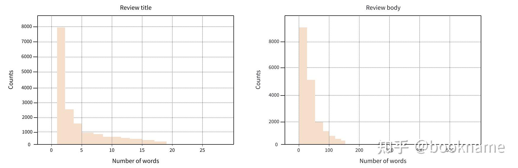

简单粗暴的解决办法就是直接过滤掉太短标题的数据，引导我们的模型生成有意义的预测摘要。因为英文和西班牙文都使用空格分割单词，因此可以简单的用空格分割标题，并使用Dataset.filter来过滤掉单词数量不大于2的数据（过滤了很多的数据呀，那么怎么能不保证过拟合，看训练过程和结果吧！）。

现在准备好了语料，下面从Hub上选择模型，并进行微调！

其实，文本摘要也是一种序列到序列任务，和翻译任务类似。对于摘要任务，我们已经有了一个较长评论，需要将其翻译成一个简短版本（较长评论的主题思想）。大多数用于摘要任务的Transformer模型使用encoder-decoder架构（在第1章中有介绍）。另外也有使用GPT架构的模型（decoder-only），该类模型对于少样本情况下摘要任务，效果也不错。下表列举了部分在摘要任务上常用的预训练模型。

如上表所示，大部分用于文本摘要的Transformer模型（其实在大多数任务中）都是单语言的。如果你的任务是关于"高资源"（就是语料比较丰富），例如英文或德文，则有丰富的预训练模型可用。但是对于成千的“低资源”语言就没有那么多的预训练模型可用了。幸运的是，有不少多语言模型可供选择，例如mT5和mBART（前面的m指的是multilingual）。mT5和mBART都是多语言语料上进行了预训练。与在一个语言语料上训练不同，这两个模型在超过50种语言的联合语料上进行了预训练。

本文主要使用mT5模型。mT5模型基于T5模型架构（T5是一种文本到文本框架）。所有的NLP任务都被统一建模为提示模式：例如摘要任务会在内容前面添加summarize:，这个提示用来帮助模型根据提示来调整生成的文本。如下图所示，这使得T5模型的功能极为丰富，可以通过一个模型来完成多个任务。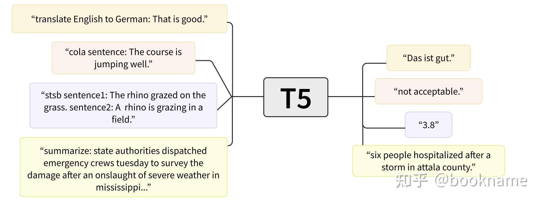

mT5没有使用前缀，但是依然具备T5的任务多样性特点，并且在多语言方面具有很多有点。现在开始选择一个模型，并且准备好训练要用的数据。

本节完成评论和标题的分词编码操作。首先加载预训练好的分词器对象。这里使用mT5-small模型，小模型主要是为了减少训练和推理时间。

在NLP项目的起步阶段，可以先在较小的数据集上试下small版本的模型。这样可以在较快时间内调试整个项目流程。一旦结果没有大问题，在后面可以扩大数据集和模型规模。

让我们在部分例子上测试mT5分词器。

好吧，从结果看，有input_ids和attention_mask分别是分词后的token id和掩码。让我们使用分词器的函数convert_ids_to_tokens()将token id转换为对应的token，如下。

由上可知，从Unicode字符_和序列结束标记可知，mT5模型的使用的是SentencePiece分词器，该分词器是一种Unigram分词器（字典由大到小的训练过程）。Unigram分词器非常适合多语言语料情况，因为SentencePiece适合处理音标、符号以及许多语言的独特语法部分。例如对于日语，没有空格字符也能很好的进行分词。

为了完成语料库的分词操作，文本和标签都需要处理。这是因为标签也是文本，其文本长度也有可能超过模型的最大输入长度（主要是指分词后的token数量）。有时候文本和标签都很长的情况下，就要对文本和标签进行截断操作。Transformer中的tokenizer可以使用一个技巧，就是as_target_tokenizer()来同时处理文本和标签。也就是在预处理函数中增加一个上下文管理器，在上下文管理器之前编码输入文本，然后在上下文管理器中处理标签，下面是mT5预处理函数的一个例子（后面直接街上map，就可以处理整个数据集）。

看下代码，观察下具体有哪些操作。首先定义了max_input_length和max_target_length两个常量，分别设置了文本和标签的最大token长度上限。因为评论文本通常远远大于标题，所以这里也相应的增加了input的长度。另外，review_body在with之前进行分词，review_title在with中进行分词。

定义了preprocess_function()函数，可以调用Dataset.map()函数来方便的进行整个数据集的处理（map()函数）。

上面代码运行一般会花掉一些时间，与数据集时间有关。下面我们看下在摘要任务中常用的指标。目前来看，很难判断一个机器生成的文本优劣（RLHF，训练一个Reward Model来判断生成文本的优劣，看来能大白魔法的只有魔法）。

注意上面函数Dataset.map()中设置参数batched=True，这样就会按照批次1000的大小来处理数据，并且使用fast tokenizer的多线程处理能力（基于Rust，所以有多线程。如果基于python，那就只有单线程）。如果硬件满足要求的话，可以在预处理的时候都使用批处理（当然也可以使用多进程进一步加速）。

和本教程中的大多数任务相比，很难直接评估文本生成（例如摘要和翻译）任务的效果。例如给定一个评论文本“I loved reading the Hunger Games”，会存在多个合理的摘要结果，例如“I loved the Hunger Games” 或 “Hunger Games is a great read”。直接文本匹配生成的摘要和标签，对于评估生成的摘要的效果不是一个很好的选择（类似RLHF，训练Reward Model来评估，应该更合理）。就算是人来评价生成摘要的优劣，依然是很困难的，因为不同的人有自己不同的写作风格（一千个人，就有一千个哈姆雷特）。

对于摘要任务，常用的指标称为ROUGE score，该指标也是比对n-gram的情况，和BLEU的区别在于其是计算召回率以及n-gram无需连续。为了测试下该指标，我们使用如下例子。

一个方法是比较两个句子的重叠部分，上例中重叠部分有6个。如果只比对重叠部分，这个也太粗糙了，因此ROUGE是计算重叠部分的精确率和召回率。

如果第一次听说精确率和召回率，也无需着急。下面会举例来讲解这两个指标（极为常见）。这两个指标在分类任务中经常使用，如果读者想详细了解精确率和召回率，可以查看scikit-learn链接guides。

对于ROUGE，召回率指的是参考标签中有多少比例被生成文本获取。如果比较文本，可以使用如下公式计算：

对比上面的例子而言，使用上面的召回率公式可得，其召回率为6/6=100%；这是因为所有的预测文本包含所有的标签。看起来还不错，但是如果我们生成的文本是 “I really really loved reading the Hunger Games all night”。这个生成文本也能得到100%的召回率，但是这个结果肯定是不好的。对于这种情况，我们还需要计算精确率，在ROUGE评价指标中，用来计算生成文本和标签的相关性。计算公式如下：

计算上面例子的精确率可得，6/10 = 60%，这个精确率小于最开始的例子中的6/7 = 86%（优劣明显呀！）。实际上计算精确率和召回率，然后用来计算F1得分（精确率和召回率的几何平均）。使用rouge_score的python包很容易完成F1得分的计算。（在国内可以加上 -i https://pypi.tuna.tsinghua.edu.cn/simple --default-timeout=2000）

然后使用evaluate库加载ROUGE计算指标函数，如下所示。

然后就可以调用函数rouge_score.compute()来计算摘要结果的得分了。

哇哦，输出了好多信息。这些信息分别表示什么呢？上面的计算其实主要包括精确率、召回率和F1得分。另外还有low、mid和high三个属性。这三个属性分别在不同文本粒度下计算ROUGE得分。rouge1基于unigram计算，这和我们前面介绍的精确率和召回率计算类似。为了验证下，我们看下ROUGE的mid值。

从结果看，精确率和召回率计算一致！那么其他ROUGE得分是什么意思呢？rouge2基于bigram计算ROUGE得分（比较成对单词出现的精确率和召回率），rougeL和rougeLsum基于最长单词序列来计算ROUGE得分。rougesum中的sum是指在整个生成摘要中的指标之和。rougeL是计算平均值。

现在已经得到了模型的计算指标（ROUGE得分）。下面开始构建一个还不错的基线模型！

文本摘要常见的基线模型就是取出文章的前3句话，通常称为lead-3基线模型。可以使用断句符号来获取这些句子范围，但是有可能会遇到像“U.S.”或“U.N.”中存在"."等断句符。所以这里使用nltk库，能够很好的处理上面的问题。使用如下命令安装nltk库。

然后下载标点符号规则。

然后，从nltk中加载分句器，并且创建一个简洁的函数来从评估文本中抽取前三句文本。使用换行符，将三个句子拼接起来，如下所示。

看起来还不错，下面从数据集中获取标签，然后使用基线数据和标签计算ROUGE得分。

在验证集上使用上述函数计算ROUGE得分，并且使用Pandas格式化输出结果。

看到rouge2得分要低于其它得分，这也说明评估文本对应的标题是比较简洁，且lead-3基线包含太多冗余信息。现在我们通过微调mT5来获取更好的基线模型。

由于Huggingface的努力，微调一个摘要模型和微调其他模型的流程基本类似（前馈和反馈）。首先加载mt5-small的checkpoint（小模型，一般的显卡可以跑的起来）。因为摘要任务是序列到序列任务，因此可以使用AutoModelForSeq2SeqLM来加载checkpoint，下面代码会自动下载和缓存权重。

老规矩，在notebook中用上面的命令登录Hub。

因为需要生成摘要来训练阶段计算ROUGE得分，因此我们这里使用Seq2SeqTraingingArguments和Seq2SeqTrainer来实现模型微调！下面定义下微调使用的参数。

上述参数中设置predict_with_generate用来在每次epoch结束时，调用生成摘要来计算ROUGE得分（评估时间比较长呀，还不如直接看loss）。解码器的解码过程是一个接一个递推的，因此需要使用模型的generate()函数（使用不带Seq2Seq的Arguments或Trainer，就无法使用该函数）。这里设置predict_with_generate=True，那么在Seq2SeqTrainer中会在评估过程中使用模型的generate函数。另外，上面代码中还设置了学习率、训练轮数和权重衰减参数等，并且设置参数save_total_limit参数，来保存最近的三个checkpoint（可怜一下磁盘空间吧，每个checkpoing独有GB级别大小）。

设置参数push_to_hub=True允许我们在训练后将模型上传到Hub（当然过程是后台自动完成，多么人性化）；并且默认使用output_dir的名称来命名该repo的名称，当然也可以通过设置参数hub_model_id来设置repo名称（也可以指定组织名称或用户名称）。例如，当需要将模型上传到huggingface-course organization，可以在Seq2SeqTrainingArguments中设置参数hub_model_id="huggingface-course/mt5-finetuned-amazon-en-es"。

下一步就是为trainer编写指标函数compute_metrics()来实现在训练过程中评估模型指标。对于摘要任务，需要在调用函数rouge_score.compute()之前完成一些解码操作，因为我们需要将预测和标签转换为字符串格式，方便计算ROUGE得分。下面的代码使用nltk的sent_tokenize()来分割摘要句子。

接下来，我们设置序列到序列任务的data collator（数据预处理器）。因为mT5是一个编码器－解码器模型，在准备解码输入和输出时需要做一些处理（将解码输入右移，得到解码输出）。解码部分的标签与常规语言模型中的处理方法类似（GPT类常用，在BART中也经常使用）。

Huggingface也很贴心的设置好了DataCollatorForSeq2Seq来完成动态补齐输入和标签的功能。实例化该data collator，需要提供tokenizer和model参数，如下。

用一些例子看看该data collator做了什么。首先我们需要移除一些列，因为它们不需要进行padding操作（不设置的话会报错）。

因为collator期望输入为一个字典列表，每个dict表示数据集中一个单独的例子，我们也希望在data collator处理之前，将数据处理为字典列表。

因为第一个例子的token长度小于第二个句子，因此会在第一个例子的输入和注意力掩码上加上[PAD]token进行补齐（对应的token_id为0）。类似的，使用-100来补齐标签（方便计算损失函数的时候忽略掉补齐部分）。最后看到decoder_input_ids是label右移一位得到的结果，且使用-100进行了长度上的补齐。

最后设置trainer，现在用前面准备的数据集、模型和data_collator进行设置。

然后开始训练。

在训练的时候，在每个epoch之后，可以看到损失函数降低以及ROUGE得分提高。一旦完成训练，可以调用函数Trainer.evaluate()来得到最终的ROUGE得分。

从得分结果来看，比lead-3基线的效果确实有一些提升。最后就是将训练结果和过程保存到Hub上，如下。

上面的代码，会将output_dir中的checkpoint和配置文件上传到Hub。通过指定tag参数，我们可以在Hub上自动设置界面，方便我们测试摘要的流水线（而不是默认的文本生成界面）。trainer.push_to_hub()的输出，是一个Git提高的URL对应的hash值，因此可以通过这个看到repo是否被改变。

上面是使用Trainer，方便是方便，但是做了很多底层的操作。如果需要更精细的控制训练过程，可以使用Accelerate来编写训练和评估过程。

使用Accelerate来微调摘要模型，与微调文本分类模型类似。最大的不同就是在训练过程中需要显性的生成预测摘要，并且计算ROUGE得分（和Seq2SeqTrainer中的调用model.generate()的操作一样），如下。（Accelerate还可以防止batch_size过大，导致显存out-of-memory错误的发生）。

首先是为每个数据分片准备DataLoader（训练集、验证集或测试集）。因为PyTorch的dataloaders需要输入格式为张量，因此将数据集格式设置为torch。

现在已经将数据集中的数据转换为tensor格式，下一步就是实例化DataCollatorForSeq2Seq。该对象需要输入模型和分词器，模型加载如下。

然后初始化data collator，并定义我们的dataloader。

下一步就是定义优化器。在我们的例子中，我们使用AdamW，Transformer类模型训练一般使用该优化器。

最后将定义好的模型、优化器和dataloaders，送入accelerate.prepare()函数中打包。

如果在TPU上训练，需要将上述要素封装在一个单独的训练函数中。

现在已经准备好的训练的主要元素，还有三件事要做：

对于学习率调度器，我们使用前面章节也使用的标准线性lr调度器（也可以使用余弦调度器）。

对于后处理，我们创建一个函数，来对生成摘要进行分句操作（根据分隔符\n）。因为这是ROUGE指标计算的格式，使用如下代码。

如果你对前面Seq2SeqTrainer中的compute_metrics()有所了解的话，其中部分代码和上面的函数代码类似。

最后在Hub上创建一个模型Repo。具体代码如下（主要使用huggingface_hub这个库来完成模型REPO的创建）。

现在可以使用该repo名称来克隆repo到本地。

然后就可以使用代码repo.push_to_hub()将模型上传。这个操作在后续代码中会用到。

摘要模型的训练循环与其他使用Accelerate库的训练循环类似，可以分为如下四个部分：

完整训练循环步骤如下所示。

运行上面代码，可以发现结果和使用Seq2SeqTrainer运行的结果类似，说明这种方式也是OK！且定制能力更强。

如果已经将模型上传到Hub，读者可以在该模型Repo下的网页上测试效果，或者使用pipeline进行测试，如下。

我们可以从测试集中挑选部分数据进行测试。首先创建一个简单的函数来展示评论、标签和生成的摘要。

让我们看下一个英文例子，如下。

看起来还不错！可以看到我们的模型已经将评论里的内容抽象出来为一个很短的文本摘要。而且更酷的是我们模型还支持双语的，下面看看在西班牙语上的表现。

上面的只要翻译过来就是很容易读懂，好像这个评论是挺容易看懂的（因为很短）。上面展示了mT5的部分魅力，也让读者感受下多语言模型的奇妙之处。

下步，我们将注意力转到一个更加复杂的任务，从头训练一个语言模型。