如何MATLAB实现用ARIMA模型输出参数实施预测 |
您所在的位置:网站首页 › ar模块是什么 › 如何MATLAB实现用ARIMA模型输出参数实施预测 |
如何MATLAB实现用ARIMA模型输出参数实施预测
|
正文
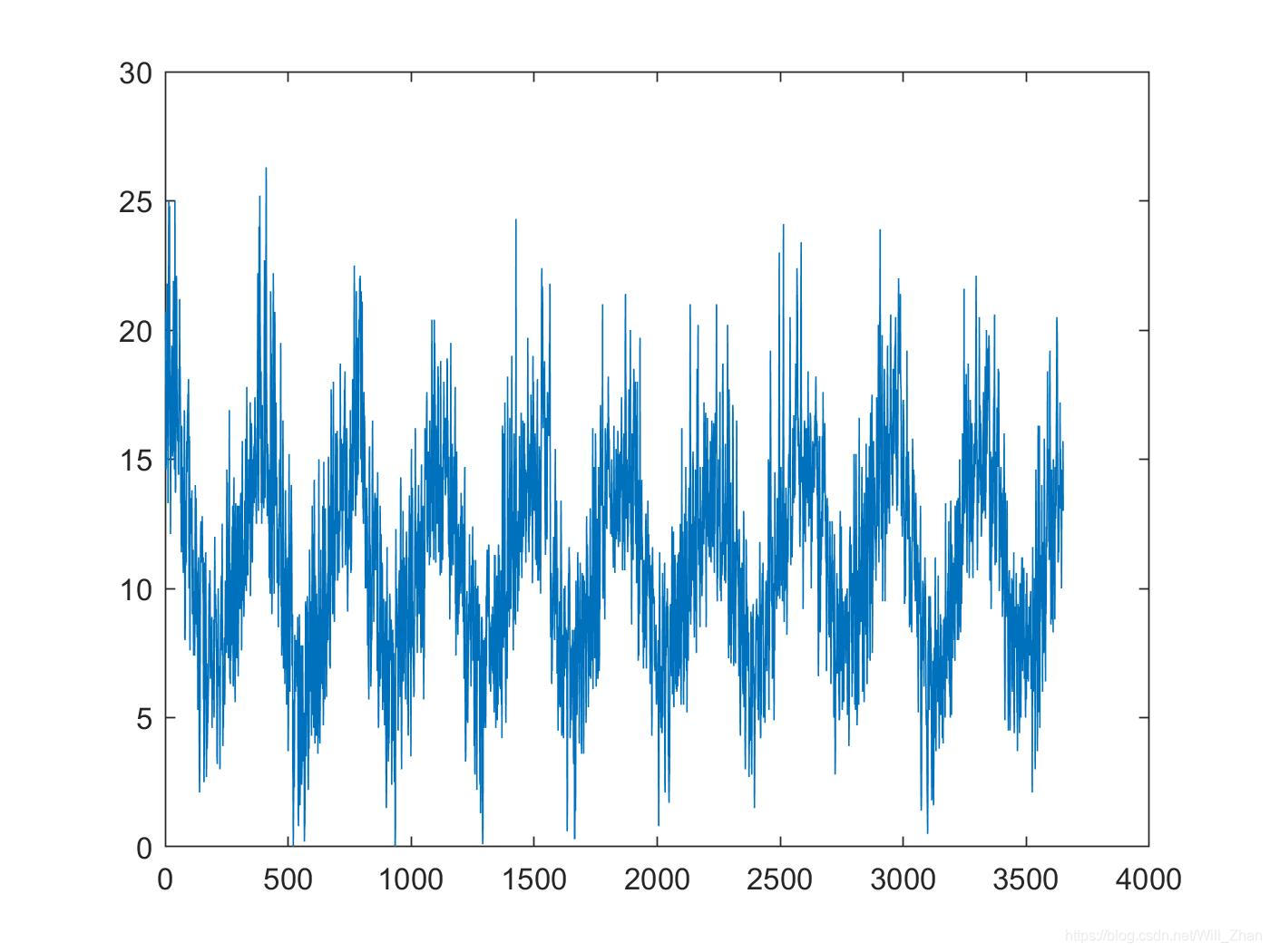
自回归(AR)模型、移动平均(MA)模型、自回归移动平均(ARMA)和自回归差分移动平均(ARIMA)模型是时间序列模型,它们主要是使用历史时间步的观测值作为回归方程的输入,以预测下一时间步的值。这是一个非常简单的想法,可以导致对一系列时间序列问题的准确预测。在本教程中,您将了解如何使用MATLAB实现时间序列预测模型。 完成本教程后,您将了解: 如何部署一个时间序列模型并进行预测。如何获取已经估计的时间序列模型的参数实施直接进行预测。结合公式更加深入了解自回归移动平均等时间序列模型。 自回归模型自回归模型,即线性回归,基于历史输入值的线性组合对输出值进行建模。 模型如下: y t = c + ϕ 1 ∗ y t − 1 + ϕ 2 ∗ y t − 2 + . . . + ϕ p ∗ y t − p + ϵ t y_t = c + \phi_1*y_{t-1}+\phi_2*y_{t-2}+...+\phi_p*y_{t-p}+\epsilon_t yt=c+ϕ1∗yt−1+ϕ2∗yt−2+...+ϕp∗yt−p+ϵt 式中: y t y_t yt是时间序列 Y \textbf{Y} Yt时刻的观测值, ϕ t \phi_t ϕt是通过对训练数据优化模型(例如最小二乘)得到的系数, ϵ t \epsilon_t ϵt是t时刻的残差, c c c为模型的常数项。 移动平均模型移动平均模型是基于移动平均过程,是一种常见的模拟时间序列过程。移动平均模型的输出变量是随机项的当前值和各种过去值线性组合。模型如下: y t = c + ϵ t + θ 1 ∗ ϵ t − 1 + θ 2 ∗ ϵ t − 2 + . . . + θ q ∗ ϵ t − q y_t = c +\epsilon_t+ \theta_1*\epsilon_{t-1}+\theta_2*\epsilon_{t-2}+...+\theta_q*\epsilon_{t-q} yt=c+ϵt+θ1∗ϵt−1+θ2∗ϵt−2+...+θq∗ϵt−q 其中 ϵ t \epsilon_t ϵt理解为均值为零的不相关正态分布的随机变量(实质是一个 innovation process)。 自回归移动平均模型自回归移动平均模型就是上述两种模型的组合,模型如下: y t = c + ϕ 1 ∗ y t − 1 + ϕ 2 ∗ y t − 2 + . . . + ϕ p ∗ y t − p + ϵ t + θ 1 ∗ ϵ t − 1 + θ 2 ∗ ϵ t − 2 + . . . + θ q ∗ ϵ t − q y_t = c + \phi_1*y_{t-1}+\phi_2*y_{t-2}+...+\phi_p*y_{t-p}+\epsilon_t+ \theta_1*\epsilon_{t-1}+\theta_2*\epsilon_{t-2}+...+\theta_q*\epsilon_{t-q} yt=c+ϕ1∗yt−1+ϕ2∗yt−2+...+ϕp∗yt−p+ϵt+θ1∗ϵt−1+θ2∗ϵt−2+...+θq∗ϵt−q 部署模型本文仅开发了简单的AR、MA、ARMA和ARIMA模型,参数没有进行优化,用于演示,参数只要稍加调整,就可获得更好的预测效果。 数据在示例中使用的最低日温度数据。 下载最低温度数据集 下载数据集到当前工作目录中,命名为“daily_minimum_temperatures.csv”将。 下面的代码将数据集作为一个数组加载。 clc; clear; % load data file = fopen("daily-minimum-temperatures.csv"); fmt = '"%u-%u-%u" %f' if file>0 series = textscan(file,fmt,'Delimiter',',','HeaderLines',1); % close the file fclose(file); end y = series{:,4}; % 仅取数值使用 plot(y);然后创建数据集的折线图: 下面演示,建立一个AR(2)模型对未来7天的值进行预测,同时写出方程,并通过取系数和滞后值的点积来计算手动输出值。 给出参数数量p = 2(即模型形式),建立模型,然后估计参数 % model AR_Order = 2; MA_Order = 0; AR2 = arima(AR_Order, 0, MA_Order); EstMdl = estimate(AR2,y);估计模型的结果直接会在窗口输出: 输出结果: 输出结果:
与AR模型类似,先建模估计参数,下面以MA(2)模型为例 % model AR_Order = 0; MA_Order = 2; MA2 = arima(AR_Order, 0, MA_Order); EstMdl = estimate(MA2,y);估计结果: 预报结果为: 使用手动获取参数按照上述公式进行预测: 这里我注意到, ϵ t − 1 \epsilon_{t-1} ϵt−1和 ϵ t − 2 \epsilon_{t-2} ϵt−2都是没法观测的,未知的。拿 ϵ t − 1 \epsilon_{t-1} ϵt−1为例,我们想要求出 ϵ t − 1 \epsilon_{t-1} ϵt−1就需要知道 y ^ t − 1 \hat{y}_{t-1} y^t−1,因为 ϵ t − 1 = y t − 1 − y ^ t − 1 \epsilon_{t-1} =y_{t-1}-\hat{y}_{t-1} ϵt−1=yt−1−y^t−1,但是 y ^ t − 1 = 11.184 + 0.75973 ∗ ϵ t − 2 + 0.3554 ∗ ϵ t − 3 \hat{y}_{t-1}=11.184 + 0.75973*\epsilon_{t-2}+0.3554*\epsilon_{t-3} y^t−1=11.184+0.75973∗ϵt−2+0.3554∗ϵt−3,从这里可以看出这是个递归的过程,需要设置初值,迭代进行确定,我这里直接将时段初的 ϵ \epsilon ϵ设置为0,然后进行模拟求出历史数据的残差序列,再实施预测,MATLAB源码可能不是这么干的,我这块也不太懂,暂时这么处理: mannual_fore = size(1:step); history = y; [len,~] = size(history); residuals = size(1:len); residuals(1:MA_Order) = 0; % 按照残差的阶数将初始值设置为0使用这个初值进行模拟求解,找出历史数据的其他初值,基本思路就是先计算模拟值,然后使用观测值和模拟计算出残差: for i=MA_Order+1:len resids = residuals(i-2:i-1); resids = rot90(resids,2); resid = history(i) - (cell2mat(EstMdl.MA)*resids' + EstMdl.Constant); residuals(i) = resid; end计算出残差序列之后,根据上述公式和残差序列计算样本外的预测值: for i=1:step resids = residuals(end-MA_Order+1:end); resids = rot90(resids,2); yhat = cell2mat(EstMdl.MA)*resids' + EstMdl.Constant; residuals = [residuals, 0]; history = [history; yhat]; mannual_fore = history(end-step+1:end); mannual_fore' end手动预测的输出结果为: ARMA模型的测试类比上述AR和MA组合即可,这里不再赘述,仅给出代码、公式和运行结果,使用的示例是ARMA(2,0,2)。 代码: clc; clear; % load data file = fopen("daily-minimum-temperatures.csv"); fmt = '"%u-%u-%u" %f' if file>0 series = textscan(file,fmt,'Delimiter',',','HeaderLines',1); % close the file fclose(file); end y = series{:,4}; %plot(y); % model AR_Order = 2; MA_Order = 2; MA1 = arima(AR_Order, 0, MA_Order); EstMdl = estimate(MA1,y); step = 10; auto_fore = forecast(EstMdl,step,'Y0',y); mannual_fore = size(1:step); history = y; [len,~] = size(history); residuals = size(1:len); max_order = max(MA_Order,AR_Order); residuals(1:max_order) = 0; for i=max_order+1:len lags = history(i-AR_Order:i-1); lags = rot90(lags,2); resids = residuals(i-MA_Order:i-1); resids = rot90(resids,2); resid = history(i) - (cell2mat(EstMdl.AR)*lags + cell2mat(EstMdl.MA)*resids' + EstMdl.Constant); residuals(i) = resid; end for i=1:step lags = history(end-AR_Order+1:end); lags = rot90(lags,2); resids = residuals(end-MA_Order+1:end); resids = rot90(resids,2); yhat = cell2mat(EstMdl.AR)*lags + cell2mat(EstMdl.MA)*resids' + EstMdl.Constant; residuals = [residuals, 0]; history = [history; yhat]; end mannual_fore = history(end-step+1:end);模型估计结果: |
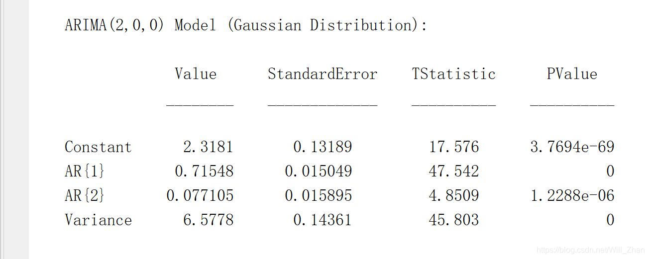 所以估计得到的方程为:
y
t
=
2.3181
+
0.71548
∗
y
t
−
1
+
0.077105
∗
y
t
−
2
+
ϵ
t
y_t = 2.3181 + 0.71548*y_{t-1}+0.077105*y_{t-2}+\epsilon_t
yt=2.3181+0.71548∗yt−1+0.077105∗yt−2+ϵt 即:
y
t
−
ϵ
t
=
y
^
t
=
2.3181
+
0.71548
∗
y
t
−
1
+
0.077105
∗
y
t
−
2
y_t-\epsilon_t=\hat{y}_t = 2.3181 + 0.71548*y_{t-1}+0.077105*y_{t-2}
yt−ϵt=y^t=2.3181+0.71548∗yt−1+0.077105∗yt−2 实施预测可以直接使用forecast()函数:
所以估计得到的方程为:
y
t
=
2.3181
+
0.71548
∗
y
t
−
1
+
0.077105
∗
y
t
−
2
+
ϵ
t
y_t = 2.3181 + 0.71548*y_{t-1}+0.077105*y_{t-2}+\epsilon_t
yt=2.3181+0.71548∗yt−1+0.077105∗yt−2+ϵt 即:
y
t
−
ϵ
t
=
y
^
t
=
2.3181
+
0.71548
∗
y
t
−
1
+
0.077105
∗
y
t
−
2
y_t-\epsilon_t=\hat{y}_t = 2.3181 + 0.71548*y_{t-1}+0.077105*y_{t-2}
yt−ϵt=y^t=2.3181+0.71548∗yt−1+0.077105∗yt−2 实施预测可以直接使用forecast()函数: 使用手动获取参数按照上述公式进行预测:
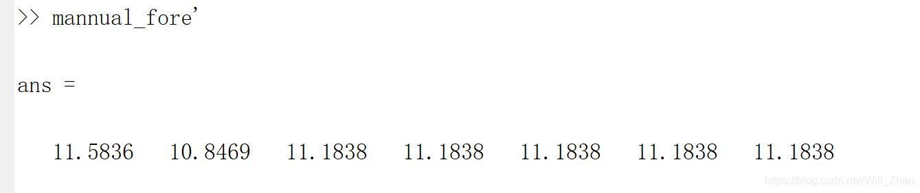
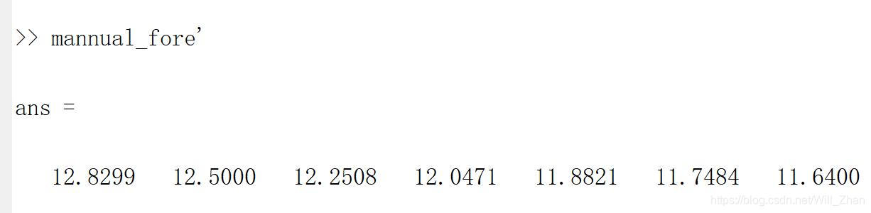 可以将上述结果进行相减,看是否是完全一致的:
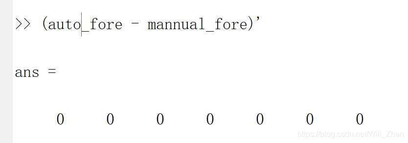 完全一致。
完全一致。 所以估计得到的方程为:
y
t
=
11.184
+
0.75973
∗
ϵ
t
−
1
+
0.3554
∗
ϵ
t
−
2
+
ϵ
t
y_t = 11.184 + 0.75973*\epsilon_{t-1}+0.3554*\epsilon_{t-2}+\epsilon_t
yt=11.184+0.75973∗ϵt−1+0.3554∗ϵt−2+ϵt 即:
y
t
−
ϵ
t
=
y
^
t
=
11.184
+
0.75973
∗
ϵ
t
−
1
+
0.3554
∗
ϵ
t
−
2
y_t-\epsilon_t=\hat{y}_t = 11.184 + 0.75973*\epsilon_{t-1}+0.3554*\epsilon_{t-2}
yt−ϵt=y^t=11.184+0.75973∗ϵt−1+0.3554∗ϵt−2 实施预测可以直接使用forecast()函数:
所以估计得到的方程为:
y
t
=
11.184
+
0.75973
∗
ϵ
t
−
1
+
0.3554
∗
ϵ
t
−
2
+
ϵ
t
y_t = 11.184 + 0.75973*\epsilon_{t-1}+0.3554*\epsilon_{t-2}+\epsilon_t
yt=11.184+0.75973∗ϵt−1+0.3554∗ϵt−2+ϵt 即:
y
t
−
ϵ
t
=
y
^
t
=
11.184
+
0.75973
∗
ϵ
t
−
1
+
0.3554
∗
ϵ
t
−
2
y_t-\epsilon_t=\hat{y}_t = 11.184 + 0.75973*\epsilon_{t-1}+0.3554*\epsilon_{t-2}
yt−ϵt=y^t=11.184+0.75973∗ϵt−1+0.3554∗ϵt−2 实施预测可以直接使用forecast()函数: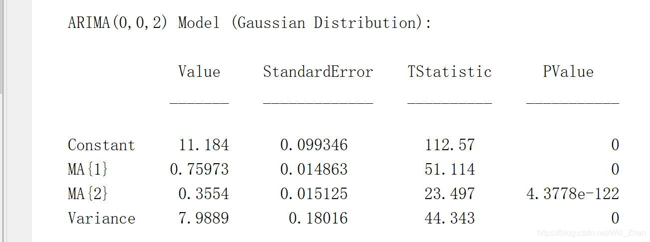 使用forecat()函数自动进行预测,结果如下:
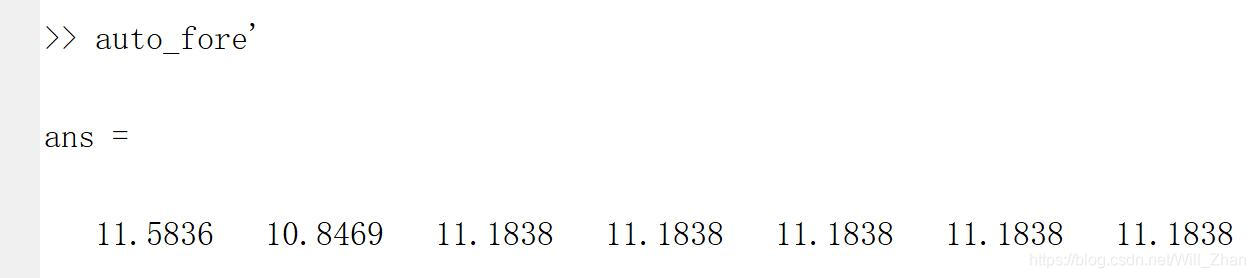
 结合上面手动和自动的预测结果可以看出,两者相同,然后将两者相减
 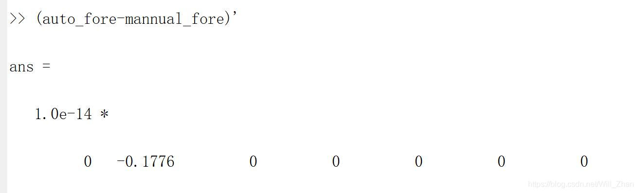 可以看出来结果不是完全一样,第二个结果有点差距,总体来看差距很小。
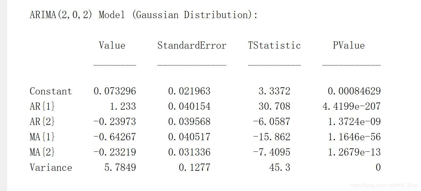 公式:
y
^
t
=
0.073296
+
1.233
∗
y
t
−
1
−
0.23973
∗
y
t
−
2
−
0.64267
∗
ϵ
t
−
1
−
0.23219
∗
ϵ
t
−
2
\hat{y}_t = 0.073296 + 1.233*y_{t-1}-0.23973*y_{t-2}-0.64267*\epsilon_{t-1}-0.23219*\epsilon_{t-2}
y^t=0.073296+1.233∗yt−1−0.23973∗yt−2−0.64267∗ϵt−1−0.23219∗ϵt−2 手动预报和自动预报结果对比:
公式:
y
^
t
=
0.073296
+
1.233
∗
y
t
−
1
−
0.23973
∗
y
t
−
2
−
0.64267
∗
ϵ
t
−
1
−
0.23219
∗
ϵ
t
−
2
\hat{y}_t = 0.073296 + 1.233*y_{t-1}-0.23973*y_{t-2}-0.64267*\epsilon_{t-1}-0.23219*\epsilon_{t-2}
y^t=0.073296+1.233∗yt−1−0.23973∗yt−2−0.64267∗ϵt−1−0.23219∗ϵt−2 手动预报和自动预报结果对比: 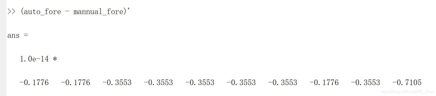 有较小的差距。
【本文地址】