从Autoencoder到VAE及其变体 |
您所在的位置:网站首页 › able的各种变形 › 从Autoencoder到VAE及其变体 |
从Autoencoder到VAE及其变体
|
本文主要是对博文1进行翻译;其中“VAE with AF Prior”小节中大部分转自博文2。侵删。 博文1:《From Autoencoder to Beta-VAE》 链接博文2:《干货 | 你的 KL 散度 vanish 了吗?》 链接目录 符号定义 1. Autoencoder, 2006 [paper] 2. Denoising Autoencoder, 2008, [paper] 3. Sparse Autoencoder, [paper] k-Sparse Autoencoder 4. Contractive Autoencoder, 2011, [paper] 5. VAE: Variational Autoencoder, 2014, [paper] 损失函数推导:ELBO/VLB(変分下界) 方式1: 根据KL散度 方式2: 根据极大似然估计进行推导 Reparameterization Trick重参数技巧 6. VAE with AF Prior, [paper] 补充:博文2:《干货 | 你的 KL 散度 vanish 了吗?》链接 7. β-VAE, 2017, [paper] 8. VQ-VAE, 2017, [paper] 9. VQ-VAE2, 2019, [paper], 比肩BigGAN的生成模型 10. TD-VAE, 2019, [paper] 符号定义
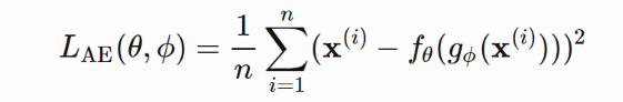
自编码器Autoencoder,是一个神经网络,采用无监督的方式学习一个Identity Function(一致变换):先对数据进行有效的压缩,然后再重建原始输入。 它由两部分组成: Encoder网络:它将原始的high-dimensional输入转换为latent low-dimensional code。输入的大小>输出的大小。Decoder网络:将latent low-dimensional code恢复为原始数据。
Encoder网络主要实现dimensionality reduction,与PCA和Matrix Factorization(矩阵因子分解)的功能类似。 Autoencoder的优化过程就是最小化reconstructed input与input之间的差异。一个好的latent representation不仅能够蕴含隐变量信息,也能很好的进行压缩和解压。
由于Autoencoder是学习一个Identity function,因此当网络的参数远远大于样本点数量时,会存在过拟合的问题。为了缓解过拟合问题,提高模型的鲁棒性,Denoising Autoencoder被提出。 Inspiration: 算法的思路来源于人类能够很好地识别对象,哪怕这个对象被部分损坏。因此,Denoise Autoencoder的目的是能够发现和捕获输入维度之间的关系,以便推断缺失的片段。 算法思路:为输入数据添加扰动,如:添加噪声/随机遮盖掉输入vector的部分值等方式,构造corrupted data;然后令Decoder恢复original input,而不是被扰动后的数据(corrupted data)。
Sparse Autoencoder(稀疏自编码) 在hidden unit activation上添加一个“sparse”约束,以避免过拟合和提高鲁棒性。它迫使模型在同一时间只有少量的隐藏单元被激活,换句话说,一个隐藏的神经元在大部分时间应该是不激活的。
回顾常用的激活函数,例如:sigmoid, tanh, relu, leaky relu, etc。当激活函数的值接近1时,神经元被激活;当接近于0时,神经元被抑制。
设第l层hidden-layer包含𝑠𝑙个神经元,那么第l层的第j个神经元的激活函数可以表示为:
k-Sparse Autoencoder(Makhzani and Frey, 2013),在bottlenect layer只保留k个神经元被激活,即:units with top k highest activations。 计算过程: 根据encoder network计算compressed code:损失函数:
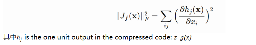
注意,反向传播时梯度只通过top k activated hidden units进行传播。 4. Contractive Autoencoder, 2011, [paper]好的表征就要具有两个特点: 可以很好地重构输入数据,如:Autoencoder, sparse autoencoder对输入数据中包含的一定程度的扰动具有鲁棒性,如:denoising autoencoder; contractive autoencoder
Contractive Autoencoder希望模型学到的表征能够具有更好地鲁棒性,对输入数据存在的小扰动具有鲁棒性。为此,在损失函数中添加一个惩罚项,确保latent representation不会对输入数据太敏感。 使用Frobenius norm of Jacobian matrix of the encoder activations with respect to the input来度量sensitivity:
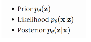
VAE其实和Autoencoder并没有非常相似,相反,它是基于变分贝叶斯(Vatiational Autoencoder)和图模型的。 与Autoencoder不同,给定一个输入样本x,我们希望得到一个latent distribution,而不是一个固定的latent representation。 我们将该分布表示成
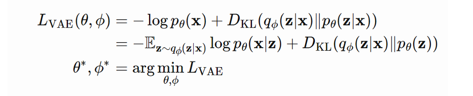
我们期望estimated posterior(近似分布) KL散度 那么,我们希望最小化
最大化上述公式的左侧式子是我们实际想要优化的目标,即:使得生成的数据似然函数最大,并且近似后验分布于实际后验分布的KL散度最小。对其取负,则可以将其转化为最小化问题:
在VAE中,该损失函数也叫作Variational Lower Bound (変分下界)。可以看到,该损失函数由两部分组成,分别为重构损失和KL损失。 那么,为什么叫变分下界呢?这是因为由于KL散度一定大于0,因此,
这样,通过最小化损失函数,我们可以最大化生成真实数据样本概率的下界。 方式2: 根据极大似然估计进行推导略;可参考CS294_158 Lecture04. Reparameterization Trick重参数技巧
论文内容:利用Autoregressive flow(AF)和Inverse Autoregressive flow (IAF)来生成先验分布。 具体实现:
损失函数:
当 VAE 和强如RNN/PixelCNN 这样的autoregressive models 在一起训练时,会出现糟糕的 “KL-vanishing problem”,或者说是 “posterior collapse”。 什么会导致KL-Vanishing呢? 回顾VAE的损失函数(如下所示),损失函数由虫谷损失和KL损失两部分组成。我们的目标是最小化损失函数,即:最小化KL的同时,最小化重构损失:
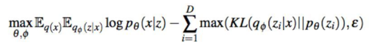
如何应对KL-Vanishing? 答案:两种策略,分别是从KL损失出发和从重构损失出发。 从KL损失出发 1. KL cost annealing: KL cost annealing 在使用上非常简单,只需要在 KL 项上乘以一个权重系数,训练刚开始的时候系数大小为0,给 q(z|x) 多一点时间学会把 x 的信息 encode 到 z 里,再随着训练 step 的增加逐渐系数增大到 1。通常搭配 word drop-out(下面有介绍)一起使用效果最佳。 代表论文:《Generating sentences from a continuous space》. CONLL 2016. 优点:代码改动很小 缺点:需要针对不同数据集调整增大的速度。推荐作为baseline 2. Free Bits: Free Bits 的想法也非常简单,为了能让更多的信息被 encode 到latent variable 里,我们让KL 项的每一维都“保留一点空间”。具体来说,如果这一维的 KL 值太小,我们就不去碰它,等到它增大超过一个阈值再优化。由此可得损失函数是:
当然,我们也可以在整个KL 上控制而不用细分到每一维度,但是这可能会导致只有很少的维度在起作用,z 的绝大部分维度并没有包含 x 的信息。 代表论文:《Improving variationalinference with inverse autoregressive flow》. NIPS 2016. 优点:Free Bits的方法操作简单 缺点:阈值 ε 也是要不断尝试的,我个人建议选取比如5左右的一个相对较小值。 3. Normalizing Flow Normalizing flow 的思想有很多变种,包括 Autoregressive Flow、Inverse Autoregressive Flow 等等。核心思想是我们先从一个简单分布采样 latent variable's latent vairable,接着通过不断迭代可逆的转换让latent variable 更为flexible。这类方法大多是为了得到一个更好的 posterior,毕竟直接用 Gaussian 建模现实问题是不够准确的。其目的是使得latent vairable的先验分布和后验分布更flexible,更复杂。但是方法复杂度较高,一个可行的替代方案是我们可以用 adversarial learning 的思想来学习 posterior,这里不多做展开。 代表论文:《Variational lossy autoencoder》. ICLR 2017. 优点:不再局限于高斯分布 缺点:方法复杂度较高 4. Auxiliary Autoencoder //待学习 代表论文: 《Improving Variational Encoder-Decoders in Dialogue Generation》. AAAI 2018. 《Z-Forcing: Training Stochastic Recurrent Networks》. NIPS 2017 从重构损失出发 1. Word drop-out Word drop-out 是典型的弱化 decoder 的方法。在训练阶段,我们将decoder 的部分输入词替换为UNK,也就是说 RNN 无法仅依靠前面的生成的词来预测下一个词了,因此需要去多依赖 z。非常有趣的一点在于,这种弱化decoder 方法还带来了性能上的提升,在 ICLR 的《Data noising as smoothing inneural network language models》文中将 Word drop-out 证明为神经网络的平滑技术,因此大家可以放心使用。 代表论文:《Generating sentences from a continuous space》. CONLL 2016. 2. CNN Decoder 既然RNN 有问题,那不妨把目光放到 CNN 上。如果只用传统的CNN 可能 contextual capacity 较差,因此可以使用 Dilated CNN decoder,通过调整 CNN 的宽度,从最弱的 Bag-of-words model 到最强的LSTM ,Dilated CNN decoder 都可以无限逼近,因此不断尝试总可以找到最合适的,方法效果也非常的好。 代表论文:《Improved Variational Autoencoders for Text Modeling using Dilated Convolutions》. ICML 2017.
3. Additional Loss 通过引入额外的 loss,例如让 z 额外去预测哪些单词会出现,因此也被称为 bag-of-words loss。之所以将其归类为第二类,因为这个方法可以看做是增大了 reconstruction 的权重,让 model 更多去关注优化reconstruction 项而不是KL。这个方法也可以非常有效避免 KL-vanishing。 代表论文:《Learning discourse-level diversity for neural dialog models using conditional variational autoencoders》.ACL 2017. 7. β-VAE, 2017, [paper]如果latent representation z的每个变量都只对一个生成因子敏感,对其他因子相对不变,我们称这个表征是disentangled或者factorized。Disentangled representation的好处在于:具有良好的可解释性,并且可以很容易的泛化到其他的task。 例如:在人脸数据集上训练的一个模型,可能捕获gentle, skin, hair color, hair length, 是否戴眼镜等等相对独立的factors。这中disentangled representation对人脸生成任务非常有帮助。 β-VAE是VAE的一个变体,其主要目标是强调发现disentangled latent factors. 和VAE一样,也是希望maximize the probability of generating real data, while keeping the distance between the real prior distribution and the approximate posterior distribution small (say, under a small constant δ):
8. VQ-VAE, 2017, [paper] VQ-VAE: Vector Quantized-Variational Autoencoder,相对于VAE,VQ-VAE模型的学习一个discrete latent variable by the encoder, 而不是连续的,因为离散的latent表征更适合一些实际场景或问题,如:语言、语音、推断等;VQ-VAE的先验分布是learnable,而不是固定的。 VQ-VAE的核心在于Vector Quantization (VQ): a method to map K-dimensional vectors into a finite set of "code" vectors. 使得先验分布和后验分布是categorial, 而不是连续的。该过程类似KNN算法,为每个feature vector寻找最近的code,并将其替换成该code。
VQ-VAE架构:
学习过程和损失函数:损失函数由三部分组成,包括:
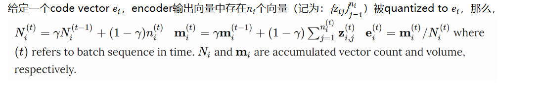
如何更新codebook中的code vector? 答案:使用 EMA (exponential moving average)算法。
训练过程分为两个阶段: 首先,按照如上损失函数训练VQ-VAE然后,基于现有输入,利用VQ-VAE的encoder+VQ模块生成一个数据集,并用它来训练PixelCNN,用来表示先验概率p(z)。采样过程: 利用训练好的pixelCNN生成latent representation将其输入到decoder中 ,生成样本 9. VQ-VAE2, 2019, [paper], 比肩BigGAN的生成模型相比于VQ-VAE,VQ-VAE2引入multi-scale hierarchical oragnization of VQ-VAE,并利用更加强大的self-attention autogressive model来学习隐变量的先验分布。 Top-level:对global information进行建模,依赖于bottom latent code,学习它们之间的关系。 输出特征大小:如果输入为256*256维度,则将其缩小8倍,得到32*32的输出Bottom Level:对local information进行建模,如纹理 输出特征大小:如果输入为256*256维度,则将其缩小4倍,得到64*64的输出
训练过程:两阶段 Stage1: train a hierarchical VQ-VAE. The design of hierarchical latent variables intends to separate local patterns (i.e., texture) from global information (i.e., object shapes). The training of the larger bottom level codebook is conditioned on the smaller top level code too, so that it does not have to learn everything from scratch.Stage2: learn a prior over the latent discrete codebook so that we sample from it and generate images. In this way, the decoder can receive input vectors sampled from a similar distribution as the one in training. A powerful autoregressive model enhanced with multi-headed self-attention layers is used to capture the prior distribution (like PixelSNAIL; Chen et al 2017).
// TO DO
|


 Vanila VAE中,假设先验分布为N(0, I),那么每个近似后验分布都应该向先验分布靠齐,则其损失函数的KL散度项变为:
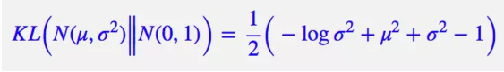


【本文地址】